| person | wage | education | female |
|---|---|---|---|
| 1 | 10.40 | 12 | 0 |
| 2 | 18.68 | 16 | 0 |
| 3 | 12.44 | 14 | 1 |
| 4 | 54.73 | 18 | 0 |
| 5 | 24.27 | 14 | 0 |
| 6 | 24.41 | 12 | 1 |
1 Data
Statistics uses observed data to learn about unknown characteristics of a population.
We begin by describing how datasets are organized and why observations are modeled as random variables.
1.1 Data Structures
Univariate Datasets
A univariate dataset consists of a sequence of observed values: Y_1, \ldots, Y_n. These n observations form a data vector: \boldsymbol{Y} = (Y_1, \ldots, Y_n)'. The prime in (Y_1, \ldots, Y_n)' denotes the transpose. Thus, \boldsymbol Y is a column vector.
Example: Survey of six individuals on their hourly earnings. The observed data vector is \boldsymbol{Y} = \begin{pmatrix} 10.40 \\ 18.68 \\ 12.44 \\ 54.73 \\ 24.27 \\ 24.41 \end{pmatrix}.
In statistical analysis, each observation Y_i is modeled as a random variable.
If data collection were repeated under the same conditions, Y_i could take a different value.
The six numbers above are one possible dataset. Repeated data collection would generally produce different values.
Multivariate Datasets
Typically, we observe more than one variable for each individual. Examples are hourly earnings, years of education, and gender.
Categorical variables are often encoded as dummy variables (also called indicator variables). These variables are binary.
The female dummy variable is defined as D_i = \begin{cases} 1 & \text{if person } i \text{ is female,} \\ 0 & \text{otherwise.} \end{cases}
A k-variate dataset (or multivariate dataset) contains n observation vectors: \boldsymbol X_1, \ldots, \boldsymbol X_n, where the i-th vector contains the k variables for individual i: \boldsymbol X_i = (X_{i1}, \ldots, X_{ik})'. Thus, X_{ij} represents the value of the j-th variable for individual i.
As before, the observation vectors are modeled as random.
The n observation vectors can be stacked as rows of an n \times k data matrix: \boldsymbol X = \begin{pmatrix} \boldsymbol X_1' \\ \vdots \\ \boldsymbol X_n' \end{pmatrix} = \begin{pmatrix} X_{11} & \ldots & X_{1k} \\ \vdots & \ddots & \vdots \\ X_{n1} & \ldots & X_{nk} \end{pmatrix}.
- The observation vector \boldsymbol X_i has dimension k \times 1.
- The full data matrix \boldsymbol X has dimension n \times k.
The data matrix for our example is \boldsymbol X = \begin{pmatrix} 10.40 & 12 & 0 \\ 18.68 & 16 & 0 \\ 12.44 & 14 & 1 \\ 54.73 & 18 & 0 \\ 24.27 & 14 & 0 \\ 24.41 & 12 & 1 \end{pmatrix}.
For instance, the first row corresponds to the observation vector \boldsymbol X_1 = (10.40, 12, 0)'.
Here, \boldsymbol X_i contains all variables measured for individual i.
Later, we distinguish one variable as the outcome:
- Y_i denotes the univariate outcome variable;
- \boldsymbol X_i collects the predictor variables.
For example, wage may be the outcome. The variables education and female may be predictors.
Matrix Algebra
Vector and matrix algebra provide a compact representation of multivariate data. They are also useful for implementing statistical methods.
We use basic matrix notation throughout the course.
To refresh or enhance your knowledge of matrix algebra, consult the following resources:
TipCrash Course on Matrix Algebra:
matrix.svenotto.com (in particular Sections 1–3)
Section 19.1 of the Stock and Watson textbook also provides a brief overview of matrix algebra concepts.
1.2 Statistical Framework
Data are usually generated by a process with a random component. Repeated data collection would generally produce different observations.
A population is the conceptual collection of all observations that could be generated under the conditions of interest.
A probability distribution F describes how likely the possible values are.
We treat the population as infinite. This makes the thought experiment n \to \infty meaningful.
Asymptotic analysis studies how statistical procedures behave as n increases.
We distinguish between three common data structures:
- Cross-sectional data: observations on many units at approximately one point in time;
- Time series data: observations on one unit recorded over multiple time periods;
- Panel data: observations on many units recorded over multiple time periods.
The data structure describes how observations are indexed.
A sampling scheme describes how observations are selected and whether they may be dependent.
Independent and Identically Distributed Sampling
Our benchmark is independent and identically distributed (i.i.d.) sampling, also called random sampling.
The random vectors \boldsymbol X_1, \ldots, \boldsymbol X_n have two important properties:
- Identically distributed: All random vectors have the same population distribution F.
- Independent: Observing one random vector provides no information about the others.
Example: Consider a survey in which individuals are randomly and independently selected from the same population.
We define an i.i.d. sample more formally at the beginning of Section 3.
The i.i.d. assumption is a model for the sampling process.
It is often a useful approximation. It is not automatically guaranteed when a dataset contains different individuals.
Dependent Observations
For dependent data, the distribution of each observation is not enough. The sampling scheme must also describe the joint dependence between observations.
Common forms of dependence are:
-
Clustered data
- Clusters are selected independently, but observations within the same cluster may be dependent.
- Example: a study that randomly selects many schools and observes all students in each selected school.
- Panel data often have this structure: repeated observations for the same individual, firm, or country may be dependent over time.
-
Time-series data
- Observations are ordered in time and may be dependent across nearby periods.
- Example: quarterly GDP growth for one country observed over consecutive quarters.
The i.i.d. sampling scheme is the core framework for the first part of this course.
Clustered and time-series data require different methods. We should not apply i.i.d. results to them without adjustment.
1.3 Datasets in R
Throughout the course, we use R to apply the theory.
The code prepares data, visualizes relationships, and computes the estimators introduced in the lecture.
R’s most common structure for tabular data is the data frame (data.frame):
- Observations are organized as rows.
- Variables are organized as columns.
- Columns can contain numeric or non-numeric values.
CA Schools Data
Let’s load the CASchools dataset from the AER package (“Applied Econometrics with R”).
If necessary, install the package with install.packages("AER").
  students teachers    income  read
1      195    10.90 22.690001 691.6
2      240    11.15  9.824000 660.5
3     1550    82.90  8.978000 636.3
4      243    14.00  8.978000 651.9
5     1335    71.50  9.080333 641.8
6      137     6.40 10.415000 605.7
The object variables contains the selected column names. CASchools[variables] selects these columns.
The head() command displays the first six rows.
The dataset contains observations for California school districts in 1998.
It is used throughout Sections 4–8 of Stock and Watson’s Introduction to Econometrics.
Important variables for this course include:
| Variable | Description |
|---|---|
| students | Total enrollment |
| teachers | Number of teachers |
| english | Percentage of English learners |
| lunch | Percentage receiving subsidized meals |
| expenditure | Expenditure per student |
| income | Average district income in thousands of dollars |
| read, math | Average reading and mathematics scores |
Variables can be accessed by name using the $ operator.
For example, CASchools$students returns the number of students in each district.
We create the student-teacher ratio and the average test score as follows:
# student-teacher ratio
CASchools$STR = CASchools$students/CASchools$teachers
# average of reading and mathematics scores
CASchools$score = (CASchools$read + CASchools$math)/2
Scatterplots provide an initial description of how test scores vary with other variables:
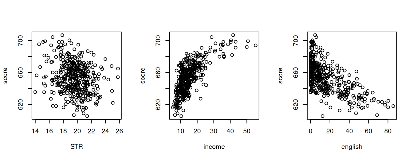
The command plot(Y ~ X, data = mydata) plots an outcome Y against a variable X.
The par() command only arranges the three plots next to each other.
CPS Data
Another dataset used throughout the course is the CPS dataset.
The dataset comes from Bruce Hansen’s textbook Econometrics.
The Current Population Survey is conducted monthly by the U.S. Census Bureau for the Bureau of Labor Statistics.
- Dataset: cps09mar.txt
- Codebook: cps09mar_description.pdf
The dataset can be downloaded and loaded using read.table():
Show download code
url = "https://users.ssc.wisc.edu/~bhansen/econometrics/cps09mar.txt"
varnames = c(
  "age", "female", "hisp", "education",
  "earnings", "hours", "week", "union",
  "uncov", "region", "race", "marital"
)
cps = read.table(url, col.names = varnames)
We first construct hourly wage and potential labor-market experience:
# hourly wage
cps$wage = cps$earnings/(cps$week * cps$hours)
# potential labor-market experience
cps$experience = pmax(cps$age - cps$education - 6, 0)
The remaining dummy variables are constructed from categories in the codebook:
Show dummy-variable code
# married dummy (see codebook for categories)
cps$married = as.numeric(
  cps$marital %in% c(1, 2, 3)
)
# Black dummy (see codebook for categories)
cps$Black = as.numeric(
  cps$race %in% c(
    2, 6, 10, 11, 12, 15, 16, 19
  )
)
# Asian dummy (see codebook for categories)
cps$Asian = as.numeric(
  cps$race %in% c(
    4, 8, 11, 13, 14, 16, 17, 18, 19
  )
)
The new commands perform three operations:
-
pmax(..., 0)replaces negative values of potential experience by zero. -
%in%checks whether each value belongs to one of the listed categories. -
as.numeric()translatesTRUEandFALSEinto the dummy values1and0.
We save the prepared dataset so that it can be loaded in later sections:
write.csv(cps, "cps.csv", row.names = FALSE)The write.csv() command saves the file in the current working directory.
It is best to use the same R Project or folder throughout the course.
Later, load the data with cps = read.csv("cps.csv").