Call:
lm(formula = wage ~ education, data = cps)

Coefficients:
(Intercept)    education
-16.448 2.898 6 Effects
6.1 Marginal Effects
Consider the regression model of hourly wage on education (years of schooling), \text{wage}_i = \beta_1 + \beta_2 \text{edu}_i + u_i, \quad i=1, \ldots, n, where the exogeneity assumption holds: E[u_i | \text{edu}_i] = 0.
The population regression function, which gives the conditional expectation of wage given education, can be derived as: \begin{align*} m(\text{edu}_i) &= E[\text{wage}_i | \text{edu}_i] \\ &= \beta_1 + \beta_2 \cdot \text{edu}_i + E[u_i | \text{edu}_i] \\ &= \beta_1 + \beta_2 \cdot \text{edu}_i \end{align*}
Thus, the average wage level of all individuals with z years of schooling is: m(z) = \beta_1 + \beta_2 \cdot z.
Interpretation of Coefficients
In the linear regression model Y_i = \boldsymbol X_i'\boldsymbol \beta + u_i, the coefficient vector \boldsymbol \beta captures the way the conditional mean of Y_i changes with the regressors \boldsymbol X_i. Under the exogeneity assumption, we have E[Y_i | \boldsymbol X_i] = \boldsymbol X_i'\boldsymbol \beta = \beta_1 + \beta_2 X_{i2} + \ldots + \beta_k X_{ik}.
This linearity allows for a simple interpretation. The coefficient \beta_j represents the partial derivative of the conditional mean with respect to X_{ij}: \frac{\partial E[Y_i | \boldsymbol X_i]}{\partial X_{ij}} = \beta_j.
This means that \beta_j measures the marginal effect of a one-unit increase in X_{ij} on the expected value of Y_i, holding all other variables constant.
If X_{ij} is a dummy variable (i.e., binary), then \beta_j measures the discrete change in E[Y_i | \boldsymbol X_i] when X_{ij} changes from 0 to 1.
For our wage-education example, the marginal effect of education is: \frac{\partial E[\text{wage}_i | \text{edu}_i]}{\partial \text{edu}_i} = \beta_2.
This population marginal effect parameter can be estimated using OLS:
Interpretation: People with one more year of education are paid on average $2.90 USD more per hour than people with one year less of education, assuming the exogeneity condition holds.
Correlation vs. Causation
The coefficient \beta_2 describes the correlative relationship between education and wages, not necessarily a causal one. To see this connection to correlation, consider the covariance of the two variables: \begin{align*} Cov(\text{wage}_i, \text{edu}_i) &= Cov(\beta_1 + \beta_2 \cdot \text{edu}_i + u_i, \text{edu}_i) \\ &= Cov(\beta_1 + \beta_2 \cdot \text{edu}_i, \text{edu}_i) + Cov(u_i, \text{edu}_i) \\ \end{align*}
The term Cov(u_i, \text{edu}_i) equals zero due to the exogeneity assumption. To see this, recall that E[u_i] = E[E[u_i|\text{edu}_i]] = 0 by the LIE, and similarly E[u_i \text{edu}_i] = E[E[u_i \text{edu}_i|\text{edu}_i]] = E[E[u_i|\text{edu}_i] \text{edu}_i] = 0, which implies Cov(u_i, \text{edu}_i) = E[u_i\text{edu}_i] - E[u_i] \cdot E[\text{edu}_i] = 0
The coefficient \beta_2 is thus proportional to the population correlation coefficient: \beta_2 = \frac{Cov(\text{wage}_i, \text{edu}_i)}{Var(\text{edu}_i)} = Corr(\text{wage}_i, \text{edu}_i) \cdot \frac{sd(\text{wage}_i)}{sd(\text{edu}_i)}.
The marginal effect is a correlative effect and does not necessarily reveal the source of the higher wage levels for people with more education.
Regression relationships do not necessarily imply causal relationships.
People with more education may earn more for various reasons:
- They might be naturally more talented or capable
- They might come from wealthier families with better connections
- They might have access to better resources and opportunities
- Education itself might actually increase productivity and earnings
The coefficient \beta_2 measures how strongly education and earnings are correlated, but this association could be due to other factors that correlate with both wages and education, such as:
- Family background (parental education, family income, ethnicity)
- Personal background (gender, intelligence, motivation)
Remember: Correlation does not imply causation!
Omitted Variable Bias
To understand the causal effect of an additional year of education on wages, it is crucial to consider the influence of family and personal background. These factors, if not included in our analysis, are known as omitted variables. An omitted variable is one that:
- is correlated with the dependent variable (\text{wage}_i, in this scenario)
- is correlated with the regressor of interest (\text{edu}_i)
- is omitted in the regression
The presence of omitted variables means that we cannot be sure that the regression relationship between education and wages is purely causal. We say that we have omitted variable bias for the causal effect of the regressor of interest.
The coefficient \beta_2 in the simple regression model measures the correlative or marginal effect, not the causal effect. This must always be kept in mind when interpreting regression coefficients.
Control Variables
We can include control variables in the linear regression model to reduce omitted variable bias so that we can interpret \beta_2 as a ceteris paribus marginal effect (ceteris paribus means holding other variables constant).
For example, let’s include years of experience as well as ethnic identity and gender dummy variables for Black and female: \text{wage}_i = \beta_1 + \beta_2 \text{edu}_i +\beta_3 \text{exper}_i + \beta_4 \text{Black}_i + \beta_5 \text{fem}_i + u_i.
In this case, \beta_2 = \frac{\partial E[\text{wage}_i | \text{edu}_i, \text{exper}_i, \text{Black}_i, \text{fem}_i]}{\partial \text{edu}_i} is the marginal effect of education on expected wages, holding experience, ethnic identity, and gender fixed.
lm(wage ~ education + experience + Black + female, data = cps)
Call:
lm(formula = wage ~ education + experience + Black + female,
    data = cps)

Coefficients:
(Intercept)    education   experience        Black       female
   -21.7089       3.1350       0.2443      -2.8554      -7.4363
Interpretation of coefficients:
- Education: Given the same experience, ethnic identity (whether the individual identifies as Black), and gender, people with one more year of education are paid on average $3.14 USD more than people with one year less of education.
- Experience: Each additional year of experience is associated with an average wage increase of $0.24 USD per hour, holding other factors constant.
- Black: Black workers earn on average $2.86 USD less per hour than non-Black workers with the same education, experience, and gender.
- Female: Women earn on average $7.43 USD less per hour than men with the same education, experience, and ethnic identity.
Note: This regression does not control for other unobservable characteristics (such as ability) or variables not included in the regression (such as quality of education), so omitted variable bias may still be present.
Good vs. Bad Controls
It’s important to recognize that control variables are always selected with respect to a particular regressor of interest. A researcher typically focuses on estimating the effect of one specific variable (like education), and control variables must be designed specifically for this relationship.
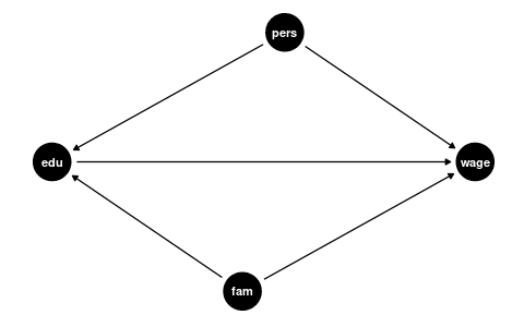
In causal inference terminology, we can distinguish between different types of variables:
- Confounders: Variables that affect both the regressor of interest and the outcome. These are good controls because they help isolate the causal effect of interest.
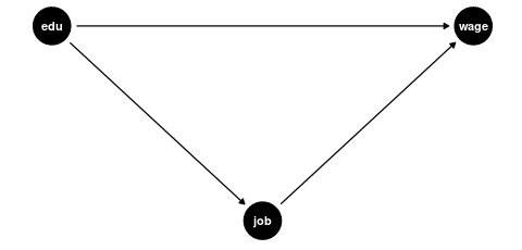
- Mediators: Variables through which the regressor of interest affects the outcome. Controlling for mediators can block part of the causal effect we’re trying to estimate.
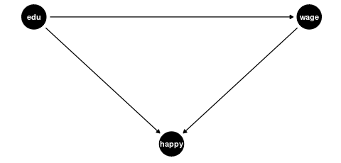
- Colliders: Variables that are affected by both the regressor of interest and the outcome (or by factors that determine the outcome). Controlling for colliders can create spurious associations.
Confounders
Examples of good controls (confounders) for education are:
- Parental education level (affects both a person’s education and their wage potential)
- Region of residence (geographic factors can influence education access and job markets)
- Family socioeconomic background (affects educational opportunities and wage potential)

Mediators and Colliders
Examples of bad controls include:
-
Mediators: Variables that are part of the causal pathway from education to wages
- Current job position (education → job position → wage)
- Professional sector (education may determine which sector someone works in)
- Number of professional certifications (likely a result of education level)
-
Colliders: Variables affected by both education and wages (or their determinants)
- Happiness/life satisfaction (might be affected independently by both education and wages)
- Work-life balance (both education and wages might affect this independently)
Bad controls create two problems:
- Statistical issue: High correlation with the variable of interest (like education) causes high variance in the coefficient estimate (high collinearity).
- Causal inference issue: They distort the relationship we’re trying to estimate by either blocking part of the causal effect (mediators) or creating artificial associations (colliders).
Good control variables are typically determined before the level of education is determined, while bad controls are often outcomes of the education process itself or are jointly determined with wages.
The appropriate choice of control variables requires not just statistical knowledge but also subject-matter expertise about the causal structure of the relationships being studied.
6.2 Application: Class Size Effect
Let’s apply these concepts to a real-world research question: How does class size affect student performance?
Recall the CASchools dataset used in the Stock and Watson textbook, which contains information on California school characteristics:
data(CASchools, package = "AER")
CASchools$STR = CASchools$students/CASchools$teachers
CASchools$score = (CASchools$read+CASchools$math)/2
We are interested in the effect of the student-teacher ratio STR (class size) on the average test score score. Following our previous discussion on causal inference, we need to consider potential confounding factors that might affect both class sizes and test scores.
Control Strategy
Let’s examine several control variables:
-
english: proportion of students whose primary language is not English. -
lunch: proportion of students eligible for free/reduced-price meals. -
expenditure: total expenditure per pupil.
First, we should check whether these variables are correlated with both our regressor of interest (STR) and the outcome (score):
                   STR      score     english       lunch expenditure
STR          1.0000000 -0.2263627  0.18764237  0.13520340 -0.61998216
score       -0.2263627  1.0000000 -0.64412381 -0.86877199  0.19127276
english      0.1876424 -0.6441238  1.00000000  0.65306072 -0.07139604
lunch        0.1352034 -0.8687720  0.65306072  1.00000000 -0.06103871
expenditure -0.6199822  0.1912728 -0.07139604 -0.06103871  1.00000000
The correlation matrix reveals that english, lunch, and expenditure are indeed correlated with both STR and score. This suggests they could be confounders that, if omitted, might bias our estimate of the class size effect.
Let’s implement a control strategy, adding potential confounders one by one to see how the estimated marginal effect of class size changes:
fit1 = lm(score ~ STR, data = CASchools)
fit2 = lm(score ~ STR + english, data = CASchools)
fit3 = lm(score ~ STR + english + lunch, data = CASchools)
fit4 = lm(score ~ STR + english + lunch + expenditure, data = CASchools)
library(modelsummary)
mymodels = list(fit1, fit2, fit3, fit4)
modelsummary(mymodels,
             statistic = NULL,
gof_map = c("nobs", "r.squared", "adj.r.squared", "rmse"))| (1) | (2) | (3) | (4) | |
|---|---|---|---|---|
| (Intercept) | 698.933 | 686.032 | 700.150 | 665.988 |
| STR | -2.280 | -1.101 | -0.998 | -0.235 |
| english | -0.650 | -0.122 | -0.128 | |
| lunch | -0.547 | -0.546 | ||
| expenditure | 0.004 | |||
| Num.Obs. | 420 | 420 | 420 | 420 |
| R2 | 0.051 | 0.426 | 0.775 | 0.783 |
| R2 Adj. | 0.049 | 0.424 | 0.773 | 0.781 |
| RMSE | 18.54 | 14.41 | 9.04 | 8.86 |
Interpretation of Marginal Effects
Let’s interpret the coefficients on STR from each model more precisely:
Model (1): Between two classes that differ by one student, the class with more students scores on average 2.280 points lower. This represents the unadjusted association without controlling for any confounding factors.
Model (2): Between two classes that differ by one student but have the same share of English learners, the larger class scores on average 1.101 points lower. Controlling for English learner status cuts the estimated effect by more than half.
Model (3): Between two classes that differ by one student but have the same share of English learners and and the same share of students eligible for reduced-price meals, the larger class scores on average 0.998 points lower. Adding this socioeconomic control further reduces the estimated effect slightly.
Model (4): Between two classes that differ by one student but have the same share of English learners, students with reduced meals, and per-pupil expenditure, the larger class scores on average 0.235 points lower. This represents a dramatic reduction from the previous model.
The sequential addition of controls demonstrates how sensitive the estimated marginal effect is to model specification. Each coefficient represents the partial derivative of the expected test score with respect to the student-teacher ratio, holding constant the variables included in that particular model.
Identifying Good and Bad Controls
Based on our causal framework from the previous section, we can evaluate our control variables:
-
Confounders (good controls):
englishandlunchare likely good controls because they represent pre-existing student characteristics that influence both class size assignments and test performance. For instance, schools with a higher share of immigrants or lower-income households may have on average higher class sizes and lower reading scores.
STR ← english → score
-
Mediator (bad control):
expenditureappears to be a bad control because it’s likely a mediator in the causal pathway from class size to test scores. Smaller classes mechanically increase per-pupil expenditure through higher teacher salary costs per student.
STR → expenditure → score
When we control for expenditure, we block this causal pathway and “control away” part of the effect of STR on score we actually want to measure. This explains the dramatic drop in the coefficient in Model (4) and suggests this model likely underestimates the true effect of class size.
This application demonstrates the crucial importance of thoughtful control variable selection in regression analysis. The estimated marginal effect of STR on score varies substantially depending on which variables we control for. Based on causal reasoning, we should prefer Model (3) with the appropriate confounders but without the mediator.
6.3 Polynomials
Experience and wages
A linear dependence of wages and experience is a strong assumption. We can reasonably expect a nonlinear marginal effect of another year of experience on wages. For example, the effect may be higher for workers with 5 years of experience than for those with 40 years of experience.
Polynomials can be used to specify a nonlinear regression function: \text{wage}_i = \beta_1 + \beta_2 \text{exper}_i + \beta_3 \text{exper}_i^2 + \beta_4 \text{exper}_i^3 + u_i.
    (Intercept)      experience I(experience^2) I(experience^3)
20.4159 1.2067 -0.0449 0.0004 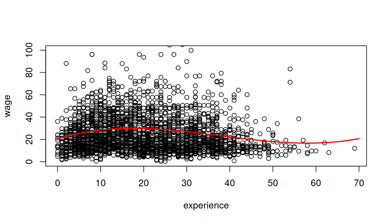
The marginal effect depends on the years of experience: \frac{\partial E[\text{wage}_i | \text{exper}_i] }{\partial \text{exper}_i} = \beta_2 + 2 \beta_3 \text{exper}_i + 3 \beta_4 \text{exper}_i^2. For instance, the additional wage for a worker with 11 years of experience compared to a worker with 10 years of experience is on average 1.2013 + 2\cdot (-0.0447) \cdot 10 + 3 \cdot 0.0004 \cdot 10^2 = 0.4273.
Income and test scores
Another example is the relationship between the income of schooling districts and their test scores.
Income and test score are positively correlated:
cor(CASchools$income, CASchools$score)[1] 0.7124308School districts with above-average income tend to achieve above-average test scores. But does a linear regression adequately model the data? Let’s compare a linear with a quadratic regression specification.
linear = lm(score ~ income, data = CASchools)
linear
Call:
lm(formula = score ~ income, data = CASchools)

Coefficients:
(Intercept)       income
    625.384        1.879
Estimated linear regression function:
\widehat{\text{score}} = 625.4 \,+ 1.88 \, \text{inc}.
Call:
lm(formula = score ~ income + I(income^2), data = CASchools)

Coefficients:
(Intercept)       income  I(income^2)
  607.30174      3.85099     -0.04231
Estimated quadratic regression function:
\widehat{\text{score}} = 607.3 \,+ 3.85 \, \text{inc} - 0.0423 \, \text{inc}^2.
# Create scatterplot
plot(score ~ income, data = CASchools,
    xlab = "District Income (thousands)",
    ylab = "Test Score")

# Add fitted curves
curve(coef(linear)[1] + coef(linear)[2]*x, add = TRUE, col = "red", lwd=2)
curve(coef(quad)[1] + coef(quad)[2]*x + coef(quad)[3]*x^2, add = TRUE, col = "blue", lwd=2)

# Add legend
legend("bottomright", c("Quadratic", "Linear"), col = c("blue", "red"), lwd = 2)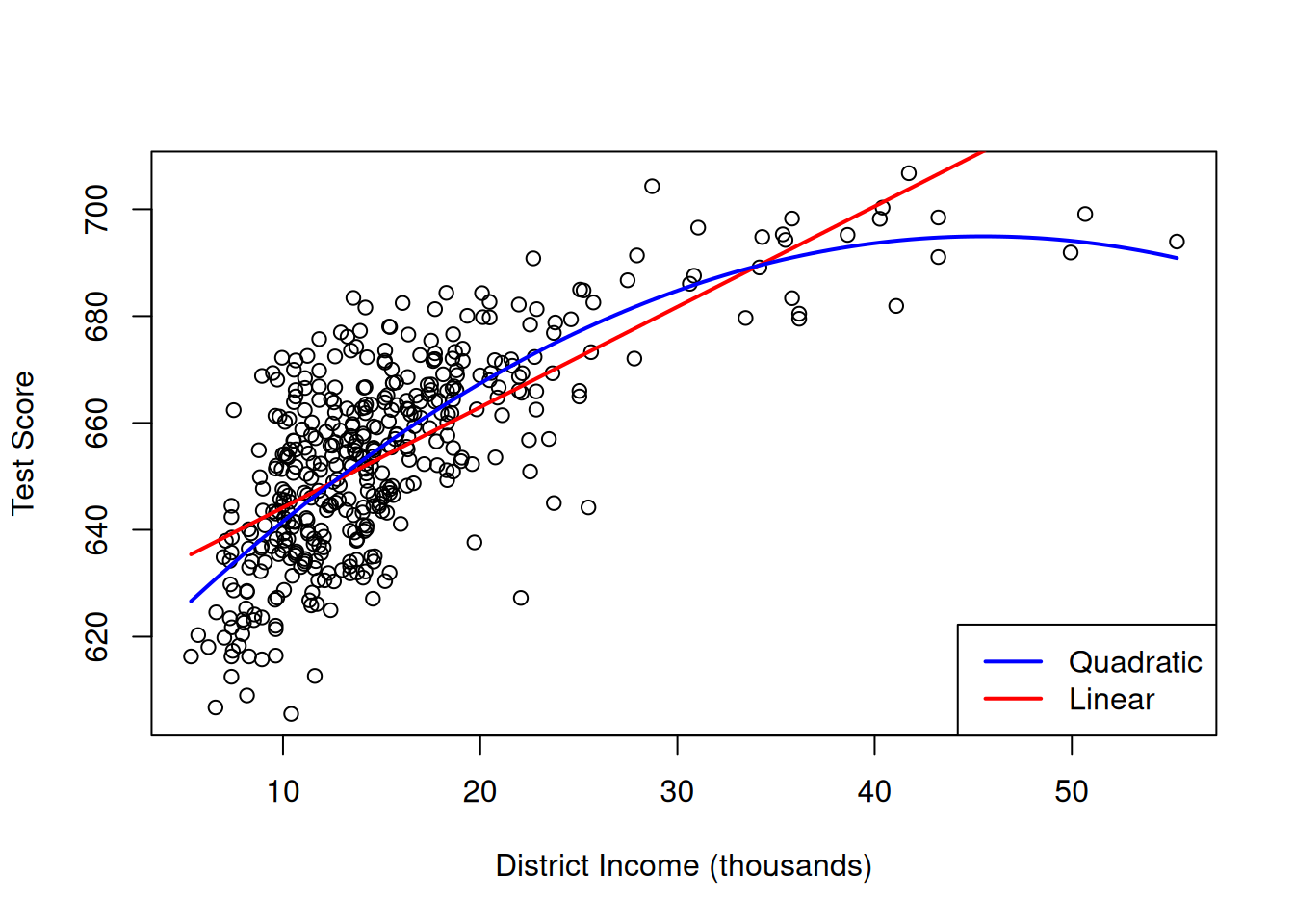
The plot shows that the linear regression line seems to overestimate the true relationship when income is either very high or very low and it tends to underestimate it for the middle income group.
The quadratic function appears to provide a better fit to the data compared to the linear function.
6.4 Logarithms
Log-income and test scores
Another approach to estimate a concave nonlinear regression function involves using a logarithmic regressor.
Call:
lm(formula = score ~ log(income), data = CASchools)

Coefficients:
(Intercept)  log(income)
     557.83        36.42
The estimated regression function is
\widehat{\text{score}} = 557.8 + 36.42 \, \log(\text{inc})
# Create scatterplot
plot(score ~ income, data = CASchools,
    xlab = "District Income (thousands)",
    ylab = "Test Score")

# Add fitted curves
curve(coef(linlog)[1] + coef(linlog)[2]*log(x), add = TRUE, col = "blue", lwd = 2)
curve(coef(linear)[1] + coef(linear)[2]*x, add = TRUE, col = "red", lwd = 2)

# Add legend
legend("bottomright", c("Linear-log", "Linear"), col = c("blue", "red"), lwd = 2)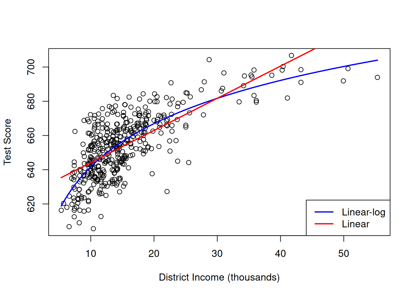
library(modelsummary)
modelsummary(list("linear" = linear, "quad" = quad, "linlog" = linlog),
             statistic = NULL,
gof_map = c("nobs", "r.squared", "adj.r.squared", "rmse"))| linear | quad | linlog | |
|---|---|---|---|
| (Intercept) | 625.384 | 607.302 | 557.832 |
| income | 1.879 | 3.851 | |
| I(income^2) | -0.042 | ||
| log(income) | 36.420 | ||
| Num.Obs. | 420 | 420 | 420 |
| R2 | 0.508 | 0.556 | 0.563 |
| R2 Adj. | 0.506 | 0.554 | 0.561 |
| RMSE | 13.35 | 12.68 | 12.59 |
We observe that the adjusted R-squared is highest for the logarithmic model, indicating that the latter is the most suitable.
The coefficients have a different interpretation.
- Assuming the linear model specification is correct, we have
E[\text{score}|\text{inc}] = \beta_1 + \beta_2 \text{inc}.
The marginal effect of
incomeonscoreis \frac{\partial E[\text{score}|\text{inc}]}{\partial \text{inc}} = \beta_2. Students from a district with $1000 higher income have on average 1.879 points higher scores. - Assuming the quadratic model specification is correct, we have
E[\text{score}|\text{inc}] = \beta_1 + \beta_2 \text{inc} + \beta_3 \text{inc}^2.
The marginal effect
incomeonscoredepends on the income level: \frac{\partial E[\text{score}|\text{inc}]}{\partial \text{inc}} = \beta_2 + 2 \beta_3 \text{inc}. When considering a district with x income, students with $1000 higher income have on average 3.85 - 0.0846x points higher scores. - Assuming the logarithmic model specification is correct, we have
E[\text{score}|\text{inc}] = \beta_1 + \beta_2 \log(\text{inc}).
The slope coefficient represents the marginal effect of
log(income)onscore: \frac{\partial E[\text{score}|\text{inc}]}{\partial \log(\text{inc})} = \beta_2. Instead, the marginal effect ofincomeonscoreis \frac{\partial E[\text{score}|\text{inc}]}{\partial \text{inc}} = \beta_2 \cdot \frac{1}{\text{inc}}, so \underbrace{\partial E[\text{score}|\text{inc}]}_{\text{absolute change}} = \beta_2 \cdot \underbrace{\frac{\partial \text{inc}}{\text{inc}}}_{\text{percentage change}}. Students from a district with 1\% higher income have on average 36.42 \cdot 1\% = 0.3642 points higher scores.
Education and log-wages
If a convex relationship is expected, we can also use a logarithmic transformation for the dependent variable:
\log(\text{wage}_i) = \beta_1 + \beta_2 \text{edu}_i + u_i
The marginal effect of education on log(wage) is
\frac{\partial E[\log(\text{wage}_i) | \text{edu}_i] }{\partial \text{edu}_i} = \beta_2.
To interpret \beta_2 in terms of changes of wage instead of log(wage), consider the following approximation:
E[\text{wage}_i | \text{edu}_i] \approx \exp(E[\log(\text{wage}_i) | \text{edu}_i]).
The left-hand expression is the conventional conditional mean, and the right-hand expression is the geometric mean. The geometric mean is slightly smaller because E[\log(Y)] < \log(E[Y]), but this difference is small unless the data is highly skewed.
The marginal effect of a change in edu on the geometric mean of wage is \frac{\partial \exp(E[\log(\text{wage}_i) | \text{edu}_i])}{\partial \text{edu}_i} = \underbrace{\exp(E[\log(\text{wage}_i) | \text{edu}_i])}_{\text{outer derivative}} \cdot \beta_2. Using the geometric mean approximation from above, we get \underbrace{\frac{\partial E[\text{wage}_i| \text{edu}_i] }{E[\text{wage}_i| \text{edu}_i]}}_{\substack{\text{percentage} \\ \text{change}}} \approx \frac{\partial \exp(E[\log(\text{wage}_i) | \text{edu}_i])}{\exp(E[\log(\text{wage}_i) | \text{edu}_i])} = \beta_2 \cdot \underbrace{\partial \text{edu}_i}_{\substack{\text{absolute} \\ \text{change}}}.
log_model
Call:
lm(formula = log(wage) ~ education, data = cps.as)

Coefficients:
(Intercept)    education
     1.3783       0.1113
Interpretation: A person with one more year of education has a wage that is 11.13% higher on average.
In addition to the linear-log and log-linear specifications, we also have the log-log specification \log(Y) = \beta_1 + \beta_2 \log(X) + u.
Log-log interpretation: When X is 1\% higher, we observe, on average, a \beta_2 \% higher Y.
6.5 Interactions
A linear regression with interaction terms: \text{wage}_i = \beta_1 + \beta_2 \text{edu}_i + \beta_3 \text{fem}_i + \beta_4 \text{marr}_i + \beta_5 (\text{marr}_i \cdot \text{fem}_i) + u_i
lm(wage ~ education + female + married + married:female, data = cps)
Call:
lm(formula = wage ~ education + female + married + married:female,
    data = cps)

Coefficients:
   (Intercept)       education          female         married  female:married
       -18.241           2.877          -3.025           7.352          -6.016
The marginal effect of gender depends on the person’s marital status:
\frac{\partial E[\text{wage}_i | \text{edu}_i, \text{fem}_i, \text{marr}_i] }{\partial \text{fem}_i} = \beta_3 + \beta_5 \text{marr}_i
Since female is a dummy variable, we interpret the marginal effect as a discrete 0 → 1 change (ceteris paribus), not literally a derivative.
Interpretation: Given the same education, unmarried women are paid on average 3.03 USD less than unmarried men, and married women are paid on average 3.03+6.02=9.05 USD less than married men.
The marginal effect of the marital status depends on the person’s gender: \frac{\partial E[\text{wage}_i | \text{edu}_i, \text{fem}_i, \text{marr}_i]} {\partial \text{marr}_i} = \beta_4 + \beta_5 \text{fem}_i Interpretation: Given the same education, married men are paid on average 7.35 USD more than unmarried men, and married women are paid on average 7.35-6.02=1.33 USD more than unmarried women.