(Intercept)   education
-16.45 2.90 4 Regression
Section 2 introduced the conditional expectation function (CEF) and the CEF error.
Section 3 showed how population moments can be estimated by sample moments.
We now combine these ideas to specify and estimate linear regression models.
4.1 From the CEF to Simple Linear Regression
Let Y_i denote hourly wage and let Z_i denote years of education.
The population CEF is m_Z(z)=E[Y_i\mid Z_i=z].
Section 2 defined the CEF error u_i=Y_i-m_Z(Z_i).
It gives the exact decomposition Y_i=m_Z(Z_i)+u_i, \qquad E[u_i\mid Z_i]=0.
Suppose the CEF is a straight line: m_Z(z)=\beta_1+\beta_2z. \tag{4.1}
Simple Linear Regression Model
The regression equation is Y_i=\beta_1+\beta_2Z_i+u_i. \tag{4.2}
The zero conditional mean condition is E[u_i\mid Z_i]=0. \tag{4.3}
At each education level, positive and negative values of u_i average to zero.
Individual wages need not lie on the line. The line describes the conditional population mean.
The condition in Equation 4.3 is also called exogeneity. Here it follows because u_i is the CEF error and the CEF in Equation 4.1 is linear.
Together, Equation 4.2 and Equation 4.3 imply \begin{align*} E[Y_i\mid Z_i] &=\beta_1+\beta_2Z_i+E[u_i\mid Z_i] \\ &=\beta_1+\beta_2Z_i. \end{align*}
Thus, the regression line is the population CEF.
4.2 Population Coefficients
The CT and LIE from Section 2 imply that Equation 4.3 gives E[r(Z_i)u_i]=0 for every function r(Z_i) for which the expectation exists.
Setting r(Z_i)=1 and r(Z_i)=Z_i gives E[u_i]=0, \qquad E[Z_iu_i]=0. \tag{4.4}
Taking expectations in Equation 4.2 gives E[Y_i]=\beta_1+\beta_2E[Z_i].
Moreover, Equation 4.4 implies \mathrm{Cov}(Z_i,u_i)=0. Therefore, \mathrm{Cov}(Y_i,Z_i) =\beta_2\mathrm{Var}(Z_i).
If Y_i and Z_i have finite second moments and \mathrm{Var}(Z_i)>0, the population coefficients are \boxed{ \beta_2 =\frac{\mathrm{Cov}(Y_i,Z_i)}{\mathrm{Var}(Z_i)}, \qquad \beta_1=E[Y_i]-\beta_2E[Z_i] }. \tag{4.5}
Thus, \beta_1 and \beta_2 are functions of population moments.
4.3 Estimating the Coefficients
Suppose (Y_1,Z_1),\ldots,(Y_n,Z_n) are an i.i.d. sample.
Substituting u_i=Y_i-\beta_1-\beta_2Z_i into Equation 4.4 gives the population equations \begin{align*} 0&=E[Y_i-\beta_1-\beta_2Z_i], \\ 0&=E[Z_i(Y_i-\beta_1-\beta_2Z_i)]. \end{align*}
Following the method of moments from Section 3, we replace each expectation by its sample average.
The estimators solve the sample equations \begin{aligned} 0&=\frac{1}{n}\sum_{i=1}^n (Y_i-\widehat\beta_1-\widehat\beta_2Z_i), \\ 0&=\frac{1}{n}\sum_{i=1}^n Z_i(Y_i-\widehat\beta_1-\widehat\beta_2Z_i). \end{aligned} \tag{4.6}
If \widehat\sigma_Z^2>0, the unique solution to Equation 4.6 is \boxed{ \widehat\beta_2 =\frac{\widehat\sigma_{YZ}}{\widehat\sigma_Z^2}, \qquad \widehat\beta_1=\overline Y-\widehat\beta_2\overline Z }. \tag{4.7}
The fitted value and OLS residual for observation i are \begin{align*} \widehat Y_i &=\widehat\beta_1+\widehat\beta_2Z_i, \\ \widehat u_i &=Y_i-\widehat Y_i. \end{align*}
The CEF error u_i uses the population CEF. Under the exact linear CEF, it is also called the regression error.
The OLS residual \widehat u_i uses estimated coefficients. We refer to it simply as the residual below.
Wage and Education
Let’s estimate the simple linear regression using the CPS sample:
Under the linear specification, the fitted regression line is \widehat m_Z(z)=-16.45+2.90z.
Thus, the fitted mean hourly wage increases by USD 2.90 for one additional year of education.
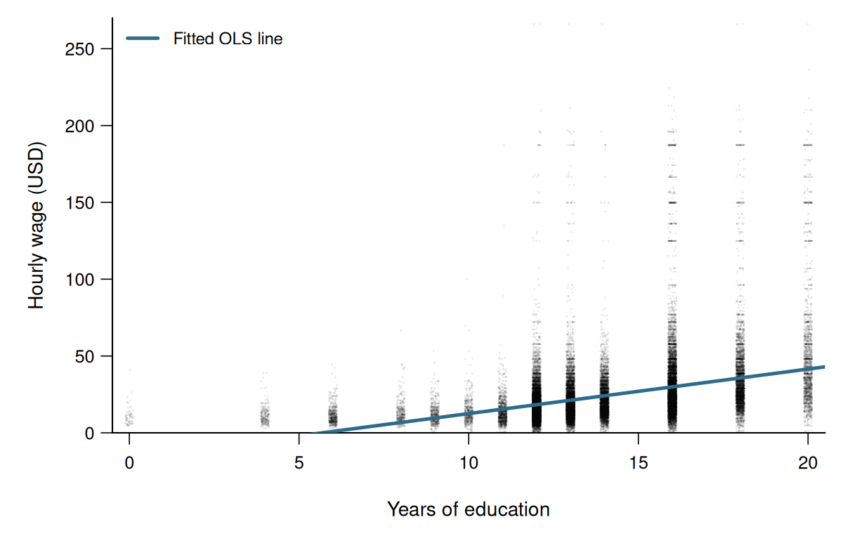
Individual wages vary substantially around the fitted line.
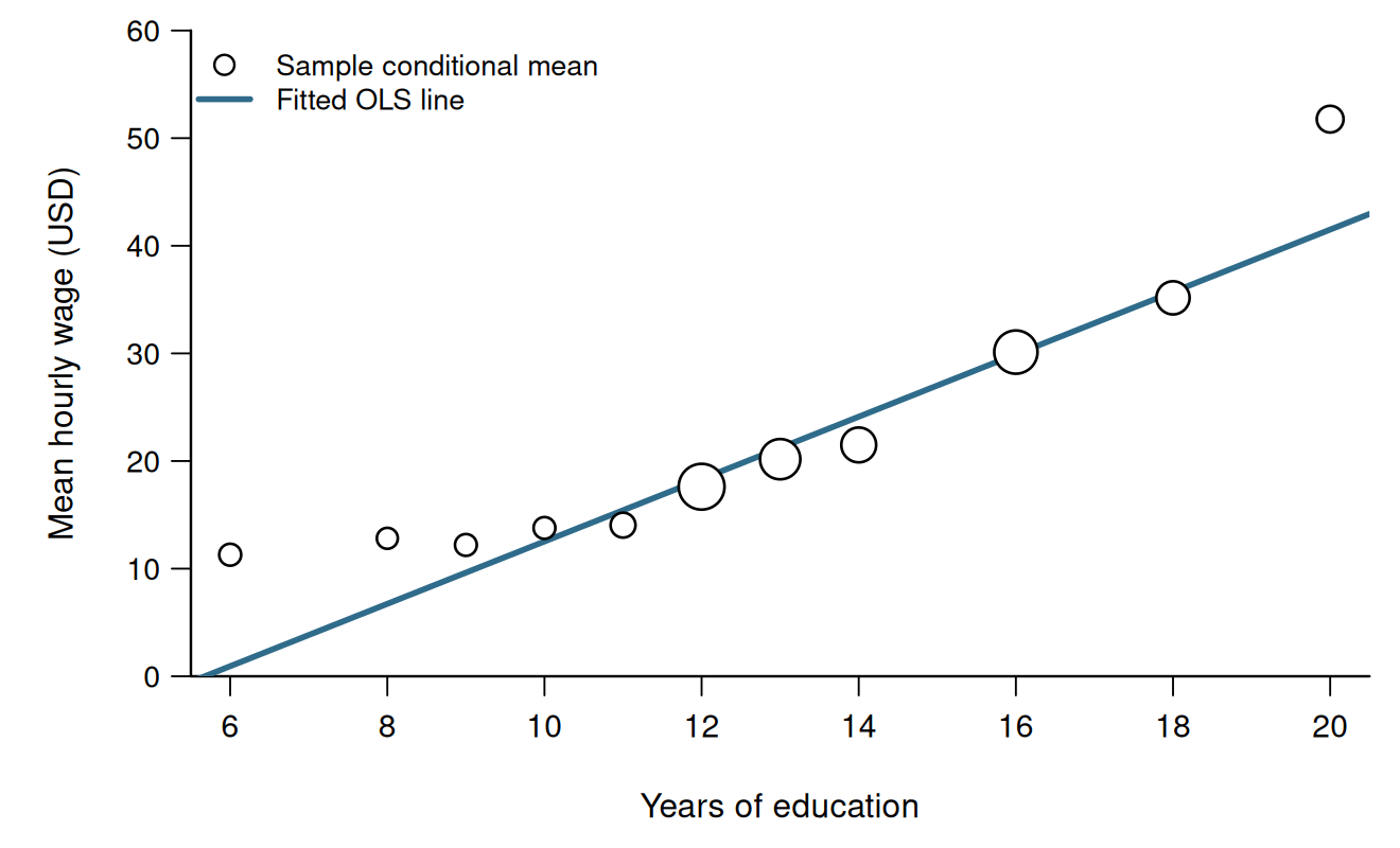
The points in Figure 4.2 are sample quantities, not values of the population CEF.
Their systematic deviations from the line may indicate that an exactly linear CEF is too restrictive. We return to this issue below.
Test Scores and Student-Teacher Ratio
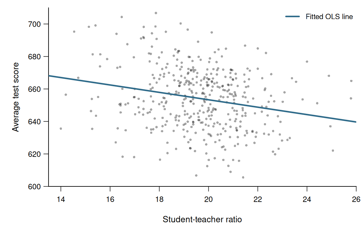
We return to the CASchools sample from Section 1.
The student-teacher ratio is the number of students per teacher. The outcome is the average of the reading and mathematics scores.
(Intercept)         STR
     698.93       -2.28
The fitted regression line is \widehat m(s)=698.93-2.28s.
A one-unit higher student-teacher ratio is associated with a 2.28-point lower fitted test score.
4.4 Why It Is Called Ordinary Least Squares
For possible coefficients b_1 and b_2, consider the sum of squared errors S_n(b_1,b_2) =\sum_{i=1}^n(Y_i-b_1-b_2Z_i)^2.
Under the condition \widehat\sigma_Z^2>0, the method-of-moments estimators in Equation 4.7 also satisfy (\widehat\beta_1,\widehat\beta_2) =\arg\min_{(b_1,b_2)\in\mathbb R^2}S_n(b_1,b_2).
The notation \arg\min returns the coefficient values that make S_n(b_1,b_2) as small as possible.
They are therefore called the ordinary least squares (OLS) estimators.
Differentiating S_n(b_1,b_2) and evaluating the first-order conditions at (b_1,b_2)=(\widehat\beta_1,\widehat\beta_2) gives \begin{align*} 0 &=\sum_{i=1}^n (Y_i-\widehat\beta_1-\widehat\beta_2Z_i) =\sum_{i=1}^n\widehat u_i, \\ 0 &=\sum_{i=1}^n Z_i(Y_i-\widehat\beta_1-\widehat\beta_2Z_i) =\sum_{i=1}^nZ_i\widehat u_i. \end{align*}
These are precisely the two sample moment conditions used above.
4.5 Multiple Linear Regression
Let \boldsymbol X_i=(1,X_{i2},\ldots,X_{ik})' contain a constant and k-1 observed regressors.
The exact linear CEF is m(\boldsymbol x) =E[Y_i\mid\boldsymbol X_i=\boldsymbol x] =\boldsymbol x'\boldsymbol\beta. \tag{4.8}
It gives the multiple linear regression model Y_i=\boldsymbol X_i'\boldsymbol\beta+u_i, \qquad E[u_i\mid\boldsymbol X_i]=0. \tag{4.9}
Regression Surface
With two nonconstant regressors, a linear CEF is a plane: E[Y_i\mid X_{i2}=x_2,X_{i3}=x_3] =\beta_1+\beta_2x_2+\beta_3x_3.
We now extend the simple regression from Section 4.3 by adding the percentage of English learners as a second regressor.
(Intercept)         STR     english
     686.03       -1.10       -0.65
The fitted regression surface is \widehat m(s,e)=686.03-1.10s-0.65e.
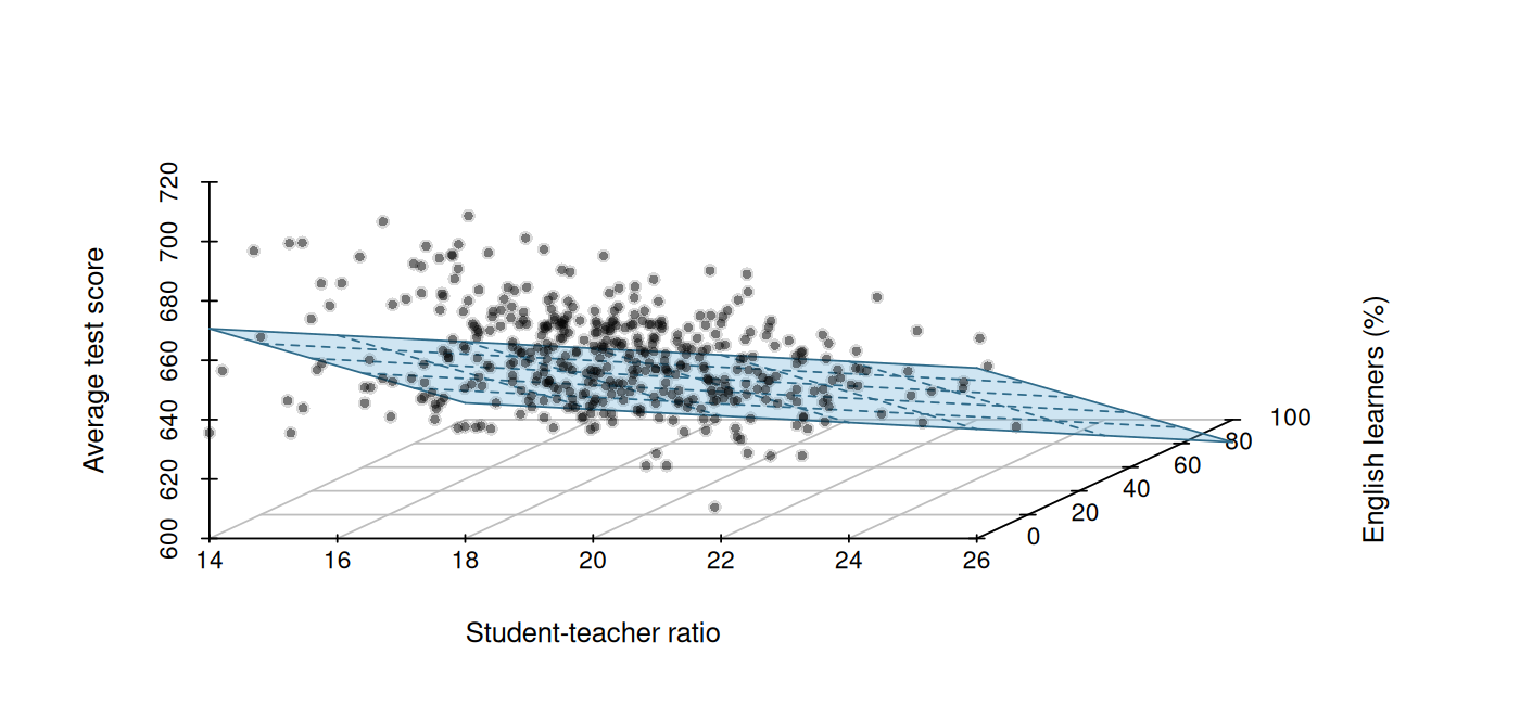
One additional student per teacher is associated with a 1.10-point lower fitted test score when the share of English learners is held fixed.
A one-percentage-point higher share of English learners is associated with a 0.65-point lower fitted score when the student-teacher ratio is held fixed.
The same interpretation applies with more regressors: one regressor changes while all the others are held fixed. The fitted function can then no longer be drawn in three dimensions.
The CT and LIE imply the population moment condition E[\boldsymbol X_iu_i]=\boldsymbol 0.
Substituting Equation 4.9 gives \begin{align*} \boldsymbol 0 &=E[\boldsymbol X_i(Y_i-\boldsymbol X_i'\boldsymbol\beta)] \\ &=E[\boldsymbol X_iY_i] -E[\boldsymbol X_i\boldsymbol X_i']\boldsymbol\beta. \end{align*}
Recall the population second moments \boldsymbol Q:=E[\boldsymbol X_i\boldsymbol X_i'], \qquad \boldsymbol q:=E[\boldsymbol X_iY_i].
The population moment condition can therefore be written as \boldsymbol q=\boldsymbol Q\boldsymbol\beta.
If \boldsymbol Q is invertible, its inverse \boldsymbol Q^{-1} exists. The population coefficient vector is then \boxed{ \begin{aligned} \boldsymbol\beta &=\boldsymbol Q^{-1}\boldsymbol q \\ &=\left(E[\boldsymbol X_i\boldsymbol X_i']\right)^{-1} E[\boldsymbol X_iY_i] \end{aligned} }. \tag{4.10}
OLS Estimator
The sample matrix \widehat{\boldsymbol Q} must be invertible to calculate the OLS estimator.
Replacing the population moments by their sample counterparts gives \begin{aligned} \widehat{\boldsymbol\beta} &=\widehat{\boldsymbol Q}^{-1}\widehat{\boldsymbol q} \\ &=\left(\frac{1}{n}\sum_{i=1}^n \boldsymbol X_i\boldsymbol X_i'\right)^{-1} \left(\frac{1}{n}\sum_{i=1}^n \boldsymbol X_iY_i\right). \end{aligned} \tag{4.11}
The data matrix stacks the row vectors \boldsymbol X_i': \boldsymbol X :=\begin{pmatrix} \boldsymbol X_1' \\ \boldsymbol X_2' \\ \vdots \\ \boldsymbol X_n' \end{pmatrix} =\begin{pmatrix} 1 & X_{12} & \cdots & X_{1k} \\ 1 & X_{22} & \cdots & X_{2k} \\ \vdots & \vdots & \ddots & \vdots \\ 1 & X_{n2} & \cdots & X_{nk} \end{pmatrix} \in\mathbb R^{n\times k}.
Let \boldsymbol Y=(Y_1,\ldots,Y_n)'\in\mathbb R^{n\times1} be the outcome vector.
Then, equivalently, \widehat{\boldsymbol\beta} =(\boldsymbol X'\boldsymbol X)^{-1}\boldsymbol X'\boldsymbol Y.
The OLS estimator also minimizes \sum_{i=1}^n(Y_i-\boldsymbol X_i'\boldsymbol b)^2 over \boldsymbol b\in\mathbb R^k.
Define the OLS residual for multiple regression \widehat u_i :=Y_i-\boldsymbol X_i'\widehat{\boldsymbol\beta}.
The residuals satisfy \frac{1}{n}\sum_{i=1}^n\boldsymbol X_i\widehat u_i =\boldsymbol 0.
The first coordinate of \boldsymbol X_i equals one. The first component of this vector equation is therefore \frac{1}{n}\sum_{i=1}^n\widehat u_i=0.
Thus, the residuals have sample mean zero.
For every nonconstant included regressor X_{ij}, j=2,\ldots,k, another component gives \frac{1}{n}\sum_{i=1}^nX_{ij}\widehat u_i=0.
Since \overline X_j is constant across observations and the residuals have sample mean zero, \frac{1}{n}\sum_{i=1}^n \overline X_j\widehat u_i =\overline X_j \frac{1}{n}\sum_{i=1}^n\widehat u_i =0.
Therefore, the cross moment is also the sample covariance: \begin{align*} \widehat\sigma_{X_j,\widehat u} &=\frac{1}{n}\sum_{i=1}^n (X_{ij}-\overline X_j)\widehat u_i \\ &=\frac{1}{n}\sum_{i=1}^nX_{ij}\widehat u_i -\overline X_j\frac{1}{n}\sum_{i=1}^n\widehat u_i =0. \end{align*}
Multicollinearity
Calculating Equation 4.11 requires an invertible sample matrix \widehat{\boldsymbol Q}.
It is not invertible when one column of the data matrix is an exact linear combination of other columns. This is called perfect multicollinearity.
In that case, the sample cannot separately determine all coefficients. Different coefficient vectors can produce the same fitted values.
Common examples include:
- including the same regressor twice,
- including the same variable in different units,
- or having k>n, so there are more coefficient columns than observations.
With near multicollinearity, the linear relation is strong but not exact. OLS can still be calculated, but the sample contains little information for separating the individual coefficients.
The resulting estimates may be sensitive and imprecise. Whether a regressor should be omitted depends on the model and the question being studied.
Dummy Variable Trap
A common source of perfect multicollinearity is the inclusion of a dummy variable for every category together with an intercept.
For example, create a dummy variable for nonmarried individuals:
(Intercept)     married  nonmarried
  19.305329    6.920139          NA
For every observation, 1=\mathrm{married}_i+\mathrm{nonmarried}_i.
The intercept is therefore an exact linear combination of the two dummy variables. The three coefficients are not uniquely determined, and R reports one of them as NA.
With an intercept and G categories, we include G-1 dummy variables. The omitted category is the reference group.
Alternatively, all G dummy variables can be included without an intercept. They then act as category-specific intercepts; in this example, they equal the two sample group means.
   married nonmarried
  26.22547   19.30533
The two coefficients equal the sample mean wage of married and nonmarried individuals, respectively.
4.6 Correct Specification and Nonlinear CEFs
A regression is linear when it is linear in its coefficients.
The CEF may therefore be nonlinear in an original regressor.
Let A_i denote years of experience. For example, m_A(a)=E[Y_i\mid A_i=a] =\gamma_1+\gamma_2a+\gamma_3a^2 \tag{4.12} is linear in \boldsymbol\gamma=(\gamma_1,\gamma_2,\gamma_3)'.
It is a multiple linear regression with regressor vector \boldsymbol X_i=(1,A_i,A_i^2)'.
The curved CEF of wage given experience from Section 2 illustrates why a quadratic term may be useful:
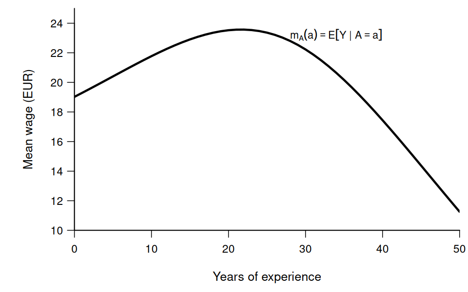
Suppose we approximate this curved CEF by the straight line a\mapsto b_1+b_2a.
Here, b_1 and b_2 are fixed coefficients of the proposed approximation. Its prediction error is v_i=Y_i-b_1-b_2A_i
The prediction error therefore has a nonzero conditional mean for at least some values of A_i: E[v_i\mid A_i]\neq0.
The straight line would then be a misspecified model for the conditional mean.
Best Linear Approximation
If the specified linear function is not the exact CEF, finite second moments and an invertible \boldsymbol Q define the best mean-squared linear approximation \boldsymbol\beta^* :=\arg\min_{\boldsymbol b\in\mathbb R^k} E[(Y_i-\boldsymbol X_i'\boldsymbol b)^2] =\boldsymbol Q^{-1}\boldsymbol q.
The corresponding linear projection error is u_i^*=Y_i-\boldsymbol X_i'\boldsymbol\beta^*.
It satisfies E[\boldsymbol X_i u_i^*]=\boldsymbol 0. In general, however, E[u_i^*\mid\boldsymbol X_i]\neq0.
Under the sampling conditions below, OLS is consistent for \boldsymbol\beta^*.
In this case, \boldsymbol X_i'\boldsymbol\beta^* approximates rather than equals the CEF.
4.7 Consistency of OLS
Section 3 established that, for a fixed number of regressors, i.i.d. sampling and finite second moments give \widehat{\boldsymbol Q}\overset{p}{\to}\boldsymbol Q, \qquad \widehat{\boldsymbol q}\overset{p}{\to}\boldsymbol q.
If \boldsymbol Q is invertible, probability-limit arithmetic gives \begin{align*} \widehat{\boldsymbol\beta} &=\widehat{\boldsymbol Q}^{-1}\widehat{\boldsymbol q} \\ &\overset{p}{\to} \boldsymbol Q^{-1}\boldsymbol q. \end{align*}
The consistency argument requires:
- i.i.d. observations (Y_i,\boldsymbol X_i')',
- finite second moments,
- an invertible population second-moment matrix \boldsymbol Q.
These conditions give consistency for \boldsymbol Q^{-1}\boldsymbol q=\boldsymbol\beta^*.
Under the regression equation and the exogeneity condition in Equation 4.9, \begin{align*} E[Y_i\mid\boldsymbol X_i] &=\boldsymbol X_i'\boldsymbol\beta +E[u_i\mid\boldsymbol X_i] \\ &=\boldsymbol X_i'\boldsymbol\beta. \end{align*}
This is the exact linear CEF in Equation 4.8. Hence \boldsymbol\beta^*=\boldsymbol\beta, and therefore \boxed{ \widehat{\boldsymbol\beta} \overset{p}{\to}\boldsymbol\beta }.
4.8 Marginal Effects
A marginal effect describes how the population CEF changes when a regressor changes, holding the other underlying regressors fixed.
If the CEF is differentiable with respect to a continuous regressor x_j, j=2,\ldots,k, its marginal effect at \boldsymbol x is ME_j(\boldsymbol x) :=\frac{\partial m(\boldsymbol x)}{\partial x_j}. \tag{4.13}
For an additive linear CEF, m(\boldsymbol x) =\beta_1+\beta_2x_2+\cdots+\beta_kx_k, we have ME_j(\boldsymbol x)=\beta_j.
The corresponding estimated marginal effect is \widehat\beta_j.
For a dummy regressor, a zero-to-one comparison is more natural than an infinitesimal change.
If D_i is the dummy and \boldsymbol C_i contains the other regressors, consider the additive linear CEF m(d,\boldsymbol c) =\beta_1+\beta_Dd+\boldsymbol c'\boldsymbol\gamma.
Formally differentiating this linear expression and calculating the zero-to-one difference both give \begin{align*} \frac{\partial m(d,\boldsymbol c)}{\partial d} &=\beta_D, \\ m(1,\boldsymbol c)-m(0,\boldsymbol c) &=\beta_D. \end{align*}
Because D_i only takes the values zero and one, the conditional-mean difference is the natural interpretation.
Treating experience as continuous, the quadratic CEF in Equation 4.12 has marginal effect \frac{\partial m_A(a)}{\partial a} =\gamma_2+2\gamma_3a.
When experience changes, both A_i and its transformation A_i^2 change. The marginal effect therefore depends on a.