             mean_wage adjusted_variance_wage    adjusted_covariance
                 23.90                 428.95                  21.83
           correlation
0.38 3 Moments
Section 2 introduced expectations as characteristics of a population distribution.
We now estimate population moments using the corresponding moments in a sample.
3.1 Random Samples
A sample of n observations is modeled by random vectors \boldsymbol W_1,\ldots,\boldsymbol W_n.
Each \boldsymbol W_i contains all variables recorded for observation i.
i.i.d. Sample
The sample is independent and identically distributed (i.i.d.) if:
- The random vectors are mutually independent across i.
- They all have the same multivariate distribution F.
Mutual independence means that the joint CDF of (\boldsymbol W_1,\ldots,\boldsymbol W_n) is the product of their individual CDFs.
It implies that every pair \boldsymbol W_i and \boldsymbol W_j, i\neq j, is independent.
Following Section 2, this has the intuitive formulation F_{\boldsymbol W_i\mid \boldsymbol W_j=\boldsymbol w_j}(\boldsymbol w_i) =F_{\boldsymbol W_i}(\boldsymbol w_i)
Knowing the realized value of \boldsymbol W_j therefore gives us no additional information about the distribution of \boldsymbol W_i.
An i.i.d. sample is also called a random sample.
The variables within \boldsymbol W_i need not be independent.
For example, wage and education may be dependent for the same person even when the observation vectors are independent across people.
The scalar sample Y_1,\ldots,Y_n is the special case with one variable per observation.
3.2 Population and Sample Moments
First consider an i.i.d. sample Y_1,\ldots,Y_n from the distribution of Y.
Population and Sample Moments
For a positive integer r with E[|Y|^r]<\infty, the r-th population moment is E[Y^r].
Its sample counterpart is the r-th sample moment \overline{Y^r} =\frac{1}{n}\sum_{i=1}^n Y_i^r.
For r=1, these are the population mean E[Y] and the sample mean \overline Y=\frac{1}{n}\sum_{i=1}^nY_i.
For the education distribution from Section 2, the first population moment is E[Y]=14.23.
The second population moment is \begin{align*} E[Y^2] &=10^2(0.06)+12^2(0.43)+14^2(0.16) \\ &\quad+16^2(0.08)+18^2(0.24)+21^2(0.03) \\ &=210.75. \end{align*}
3.3 Parameters and Estimators
We use three related terms.
- A parameter is a fixed characteristic of a population distribution, such as E[Y].
- An estimator is a function of the random sample, such as \overline Y.
- An estimate is the value of an estimator computed from an observed sample.
An estimator is itself a random variable because it depends on the random sample.
Method of Moments
The method of moments replaces population moments by their sample counterparts.
Let \boldsymbol W be a random vector and let \boldsymbol\theta\in\mathbb R^{p\times1} denote the population parameter.
Suppose \boldsymbol g(\boldsymbol W,\boldsymbol\theta)\in\mathbb R^{p\times1}.
Assume the population moment conditions uniquely determine \boldsymbol\theta: E[\boldsymbol g(\boldsymbol W,\boldsymbol\theta)]=\boldsymbol 0.
Thus, there are p moment conditions for p parameters.
Now suppose an i.i.d. sample \boldsymbol W_1,\ldots,\boldsymbol W_n is observed.
The method-of-moments estimator replaces the expectation by its sample counterpart.
It solves the p sample equations \frac{1}{n}\sum_{i=1}^n \boldsymbol g(\boldsymbol W_i,\widehat{\boldsymbol\theta}) =\boldsymbol 0, when a solution exists.
For a simple example with p=2, suppose E[Y^2]<\infty and define \mu_1=E[Y] \quad\text{and}\quad \mu_2=E[Y^2].
The parameter vector \boldsymbol\mu=(\mu_1,\mu_2)' satisfies the two population moment conditions E[Y-\mu_1]=0 \quad\text{and}\quad E[Y^2-\mu_2]=0.
Replacing the expectations by sample averages gives \overline Y-\widehat\mu_1=0 \quad\text{and}\quad \overline{Y^2}-\widehat\mu_2=0.
Their solution is \widehat{\boldsymbol\mu} =\begin{pmatrix} \widehat\mu_1 \\ \widehat\mu_2 \end{pmatrix} =\begin{pmatrix} \overline Y \\ \overline{Y^2} \end{pmatrix}.
3.4 Variance
The population variance measures dispersion around the population mean: \mathrm{Var}(Y) =E[(Y-E[Y])^2] =E[Y^2]-E[Y]^2.
Its sample counterpart is \widehat\sigma_Y^2 =\frac{1}{n}\sum_{i=1}^n(Y_i-\overline Y)^2 =\overline{Y^2}-\overline Y^2.
For the education distribution, \mathrm{Var}(Y)=210.75-14.23^2=8.26.
The population and sample standard deviations are \mathrm{sd}(Y)=\sqrt{\mathrm{Var}(Y)} \quad\text{and}\quad \widehat\sigma_Y=\sqrt{\widehat\sigma_Y^2}.
The population standard deviation is the root-mean-square distance of Y from its population mean. It can therefore be interpreted as a typical distance from the mean.
The population standard deviation of education is approximately 2.87 years.
Unlike the variance, a standard deviation is expressed in the original units of the variable.
3.5 Cross Moments
Let (Y_1,Z_1),\ldots,(Y_n,Z_n) be an i.i.d. sample from the joint distribution of (Y,Z).
Suppose Y and Z have finite second moments. The population and sample cross moments are E[YZ] \quad\text{and}\quad \overline{YZ}=\frac{1}{n}\sum_{i=1}^nY_iZ_i.
The population covariance is the central cross moment \begin{align*} \mathrm{Cov}(Y,Z) &=E[(Y-E[Y])(Z-E[Z])] \\ &=E[YZ]-E[Y]E[Z]. \end{align*}
Its sample counterpart is \begin{align*} \widehat\sigma_{YZ} &=\frac{1}{n}\sum_{i=1}^n(Y_i-\overline Y)(Z_i-\overline Z) \\ &=\overline{YZ}-\overline Y\,\overline Z. \end{align*}
Covariance depends on the units of both variables.
If both standard deviations are positive, correlation standardizes the covariance: \mathrm{Corr}(Y,Z) =\frac{\mathrm{Cov}(Y,Z)}{\mathrm{sd}(Y)\mathrm{sd}(Z)}.
If both sample standard deviations are positive, the sample correlation is r_{YZ} =\frac{\widehat\sigma_{YZ}} {\widehat\sigma_Y\widehat\sigma_Z}.
Correlation is unit-free and lies between -1 and 1.
It describes the direction and strength of a linear association.
If Y and Z are independent, then \mathrm{Cov}(Y,Z)=0. The converse does not generally hold.
Useful Rules
For random variables with finite second moments and constants a,b,c,d, \begin{align*} \mathrm{Var}(a+bY)&=b^2\mathrm{Var}(Y), \\ \mathrm{Cov}(a+bY,c+dZ)&=bd\,\mathrm{Cov}(Y,Z), \\ \mathrm{Var}(Y+Z)&=\mathrm{Var}(Y)+2\mathrm{Cov}(Y,Z)+\mathrm{Var}(Z). \end{align*}
The covariance rule is also linear in sums. For example, \mathrm{Cov}(Y+Z,X)=\mathrm{Cov}(Y,X)+\mathrm{Cov}(Z,X).
3.6 Convergence in Probability
A good estimator should be close to the population parameter when the sample size is large.
Because an estimator is random, this idea is defined using convergence in probability.
Convergence in Probability
A sequence of random variables V_n converges in probability to a constant c if, for every \epsilon>0, \lim_{n\to\infty}P(|V_n-c|>\epsilon)=0.
We write V_n\overset{p}{\to}c.
Choose any fixed distance \epsilon>0, for example \epsilon=0.05.
As n becomes large, the probability that V_n lies between c-\epsilon and c+\epsilon approaches one.
It need not equal c exactly.
This probability need not increase at every sample size. Only its limiting behavior matters.
Consistency
An estimator \widehat\theta_n is consistent for \theta if \widehat\theta_n\overset{p}{\to}\theta \quad\text{as }n\to\infty.
Thus, for any fixed precision \epsilon>0, \widehat\theta_n lies within \epsilon of \theta with probability close to one when n is sufficiently large.
The limit n\to\infty describes a sequence of increasingly large random samples from the population.
It is a theoretical device for studying whether an estimator learns the population parameter as more data become available.
3.7 Law of Large Numbers
The law of large numbers connects sample averages to population expectations.
Law of Large Numbers (LLN)
Let W_1,W_2,\ldots be i.i.d. and suppose E[|h(W_i)|]<\infty.
Then \frac{1}{n}\sum_{i=1}^n h(W_i) \overset{p}{\to}E[h(W_i)].
Setting h(W_i)=Y_i shows that the sample mean is consistent for the population mean.
Setting h(W_i)=Y_i^r shows that the r-th sample moment is consistent for the r-th population moment when E[|Y_i|^r]<\infty.
Moment conditions matter
The LLN applies to a particular function h only when E[|h(W_i)|]<\infty.
If Y is normally distributed, all polynomial moments exist: E[|Y|^s]<\infty for every positive integer s.
By contrast, if Y has a t distribution with r>1 degrees of freedom, then E[|Y|^{r-1}]<\infty \quad\text{but}\quad E[|Y|^r]=\infty.
Thus, whether the LLN applies depends on the population distribution and the moment being estimated.
For each sample size, we draw 4{,}000 independent samples of n fair coin flips.
Each sample gives one estimate \overline Y_n: the proportion of heads.
The solid black line marks E[Y]=0.5. The dashed red lines mark 0.5\pm\epsilon for \epsilon=0.05.
The red bars contain estimates for which |\overline Y_n-0.5|>0.05.
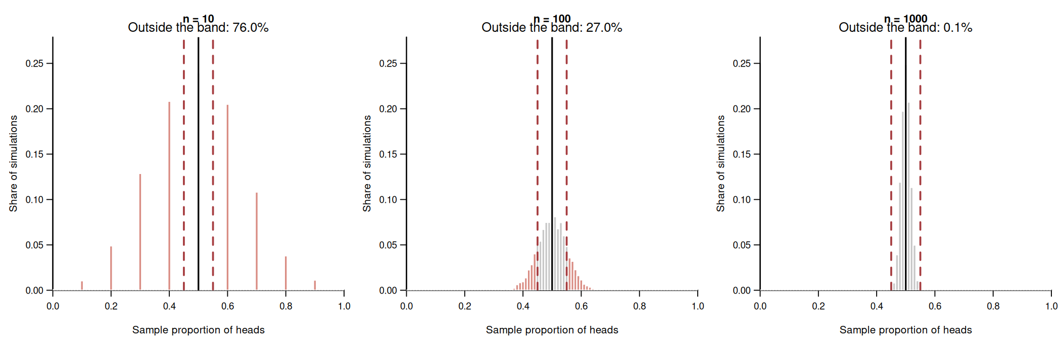
As n increases, the sampling distribution concentrates around 0.5, and the simulated share outside the fixed band decreases toward zero.
The interactive app allows other sample sizes and distributions to be explored:
Combining Probability Limits
Probability limits can be combined using the continuous mapping theorem and Slutsky’s lemma.
If V_n\overset{p}{\to}v and W_n\overset{p}{\to}w, then \begin{align*} V_n+W_n&\overset{p}{\to}v+w, \\ V_nW_n&\overset{p}{\to}vw, \\ \frac{V_n}{W_n}&\overset{p}{\to}\frac{v}{w}\quad\text{if }w\neq0. \end{align*}
More generally, if g is continuous at v, then V_n\overset{p}{\to}v \quad\Longrightarrow\quad g(V_n)\overset{p}{\to}g(v).
For example, if E[Y^2]<\infty, then \begin{align*} \widehat\sigma_Y^2 &=\overline{Y^2}-\overline Y^2 \\ &\overset{p}{\to}E[Y^2]-E[Y]^2 =\mathrm{Var}(Y). \end{align*}
Thus, the sample variance is consistent for the population variance.
The same argument gives \widehat\sigma_Y\overset{p}{\to}\mathrm{sd}(Y) \quad\text{and}\quad \widehat\sigma_{YZ}\overset{p}{\to}\mathrm{Cov}(Y,Z) under i.i.d. sampling and finite second moments.
If both population variances are positive, then r_{YZ}\overset{p}{\to}\mathrm{Corr}(Y,Z).
The i.i.d. LLN is the main case used here.
LLNs also exist for clustered and time-series data, but they require additional conditions.
We return to these sampling schemes when discussing estimation and inference in later chapters.
3.8 Multivariate Moments
Let \boldsymbol W_i=(Y_i,\boldsymbol X_i')', where Y_i is a scalar random variable and \boldsymbol X_i\in\mathbb R^{k\times1} is a random vector.
The transpose \boldsymbol X_i' has dimension 1\times k.
Thus, \boldsymbol X_i\boldsymbol X_i' is a k\times k outer product. The vector \boldsymbol X_iY_i has dimension k\times1.
The sample mean vector and its population counterpart are \overline{\boldsymbol X} =\frac{1}{n}\sum_{i=1}^n\boldsymbol X_i \quad\text{and}\quad E[\boldsymbol X_i].
The sample second-moment matrix and sample cross-moment vector are \begin{align*} \widehat{\boldsymbol Q} &=\frac{1}{n}\sum_{i=1}^n\boldsymbol X_i\boldsymbol X_i' \in\mathbb R^{k\times k}, \\ \widehat{\boldsymbol q} &=\frac{1}{n}\sum_{i=1}^n\boldsymbol X_iY_i \in\mathbb R^{k\times1}. \end{align*}
Their population counterparts are \boldsymbol Q=E[\boldsymbol X_i\boldsymbol X_i'] \quad\text{and}\quad \boldsymbol q=E[\boldsymbol X_iY_i].
Expectations and probability limits of vectors and matrices are understood component by component.
Suppose the complete observations \boldsymbol W_1,\ldots,\boldsymbol W_n are i.i.d.
If Y_i and the components of \boldsymbol X_i have finite second moments, the LLN implies \begin{align*} \overline{\boldsymbol X}&\overset{p}{\to}E[\boldsymbol X_i], \\ \widehat{\boldsymbol Q}&\overset{p}{\to}\boldsymbol Q, \\ \widehat{\boldsymbol q}&\overset{p}{\to}\boldsymbol q. \end{align*}
The population covariance matrix is \begin{align*} \mathrm{Var}(\boldsymbol X_i) &=E[(\boldsymbol X_i-E[\boldsymbol X_i]) (\boldsymbol X_i-E[\boldsymbol X_i])'] \\ &=E[\boldsymbol X_i\boldsymbol X_i'] -E[\boldsymbol X_i]E[\boldsymbol X_i]'. \end{align*}
The sample covariance matrix is \begin{align*} \widehat{\boldsymbol\Sigma} &=\frac{1}{n}\sum_{i=1}^n (\boldsymbol X_i-\overline{\boldsymbol X}) (\boldsymbol X_i-\overline{\boldsymbol X})' \\ &=\widehat{\boldsymbol Q} -\overline{\boldsymbol X}\,\overline{\boldsymbol X}'. \end{align*}
The covariance matrix centers \boldsymbol X_i around its mean; the second-moment matrix does not.
3.9 Moments in R
The sample moments defined above use n in the denominator.
The functions var() and cov() in R instead compute adjusted sample variances and covariances.
The function sd() returns the corresponding adjusted sample standard deviation.
The deviations Y_i-\overline Y sum to zero. Knowing n-1 deviations therefore determines the last one.
The adjustment accounts for this lost degree of freedom by replacing n with n-1: \begin{align*} s_Y^2 &=\frac{1}{n-1}\sum_{i=1}^n(Y_i-\overline Y)^2 =\frac{n}{n-1}\widehat\sigma_Y^2, \\ s_Y&=\sqrt{s_Y^2}, \\ s_{YZ} &=\frac{1}{n-1}\sum_{i=1}^n (Y_i-\overline Y)(Z_i-\overline Z) =\frac{n}{n-1}\widehat\sigma_{YZ}. \end{align*}
The adjustment cancels in the correlation. Thus, cor() gives the sample correlation r_{YZ} defined above.
Let’s load the CPS dataset and compute moments of wage and education:
The sample correlation between wage and education is positive.
We can obtain all pairwise correlations with cor():
dat = data.frame(
  wage = cps$wage,
  education = cps$education,
  female = cps$female
)

round(cor(dat), 2)
wage education female
wage 1.00 0.38 -0.16
education 0.38 1.00 0.04
female -0.16 0.04 1.00The sample second-moment matrix and cross-moment vector can be calculated directly.
Let the data matrix \boldsymbol X contain \boldsymbol X_i' in row i, and let \boldsymbol Y=(Y_1,\ldots,Y_n)'. Then \begin{align*} \frac{\boldsymbol X'\boldsymbol X}{n} &=\frac{1}{n}\sum_{i=1}^n\boldsymbol X_i\boldsymbol X_i' =\widehat{\boldsymbol Q}, \\ \frac{\boldsymbol X'\boldsymbol Y}{n} &=\frac{1}{n}\sum_{i=1}^n\boldsymbol X_iY_i =\widehat{\boldsymbol q}. \end{align*}
In R, t(X) computes \boldsymbol X' and %*% performs matrix multiplication.
          constant education female
constant      1.00     13.92   0.43
education    13.92    201.43   5.99
female 0.43 5.99 0.43round(qhat, 2) [,1]
constant 23.90
education 354.66
female 8.51The first column of \boldsymbol X is constant.
Therefore, the first row and column of \widehat{\boldsymbol Q} contain the sample means of the columns of \boldsymbol X.
The first element of \widehat{\boldsymbol q} is the sample mean of wage.