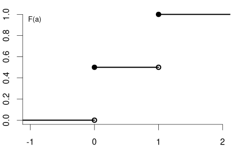
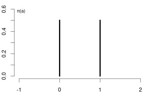
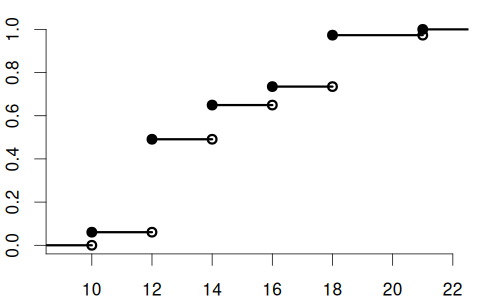
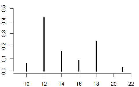
The support\mathcal Y is the set of values that Y takes with positive probability:
\mathcal Y=\{a\in\mathbb R:\pi_Y(a)>0\}.
For the education variable, \mathcal Y=\{10,12,14,16,18,21\} and
\sum_{a\in\mathcal Y}\pi_Y(a)=1.
2.3 Continuous Random Variables with a Density
A continuous random variable has a CDF without jumps. Therefore,
P(Y=a)=F_Y(a)-F_Y(a^-)=0
for every a.
Probability Density Function (PDF)
If the CDF F_Y is continuously differentiable, its PDF is obtained by differentiation:
f_Y(a)=\frac{d}{da}F_Y(a).
More generally, a nonnegative function f_Y is a PDF of Y if, for every a,
F_Y(a)=\int_{-\infty}^{a}f_Y(u)\,du.
A PDF may therefore exist even if the CDF is not differentiable at every point.
Every PDF integrates to one: \int_{-\infty}^{\infty}f_Y(u)\,du=1.
Wage per Hour
Suppose you ask a randomly selected employed person about their hourly wage in EUR.
We model wage as a continuous random variable with nonnegative values.
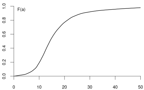
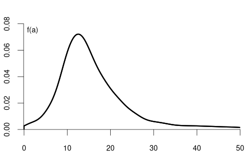
The CDF and PDF of wage may have the following form:
(a) CDF of wage
(b) PDF of wage
Figure 2.3: Wage variable: CDF (left) and PDF (right)
For a<b,
P(a<Y\leq b)=F_Y(b)-F_Y(a)=\int_a^b f_Y(u)\,du.
The PDF value f_Y(a) is not a probability. Probabilities are areas under the density over intervals.
Because point probabilities are zero, strict and non-strict interval endpoints give the same probability.
2.4 Joint and Conditional Distributions
For two random variables Y and Z, we distinguish:
The joint distribution, which describes how Y and Z behave together.
The marginal distributions, which describe Y and Z individually.
The conditional distributions, which describe one variable given information about the other.
Joint and Marginal Distributions
The joint CDF of Y and Z is
F_{Y,Z}(a,b)=P(Y\leq a,Z\leq b).
The marginal CDFs are obtained from the joint CDF: \begin{align*}
F_Y(a)&=\lim_{b\to\infty}F_{Y,Z}(a,b), \\
F_Z(b)&=\lim_{a\to\infty}F_{Y,Z}(a,b).
\end{align*}
When both variables are discrete, the joint PMF and marginal PMFs satisfy \begin{align*}
\pi_{Y,Z}(a,b)&=P(Y=a,Z=b), \\
\pi_Y(a)&=\sum_{v\in\mathcal Z}\pi_{Y,Z}(a,v), \\
\pi_Z(b)&=\sum_{u\in\mathcal Y}\pi_{Y,Z}(u,b).
\end{align*}
If (Y,Z) has a joint density f_{Y,Z}, then
F_{Y,Z}(a,b)
=\int_{-\infty}^{a}\int_{-\infty}^{b}f_{Y,Z}(u,v)\,dv\,du.
The corresponding marginal densities are \begin{align*}
f_Y(a)&=\int_{-\infty}^{\infty}f_{Y,Z}(a,v)\,dv, \\
f_Z(b)&=\int_{-\infty}^{\infty}f_{Y,Z}(u,b)\,du.
\end{align*}
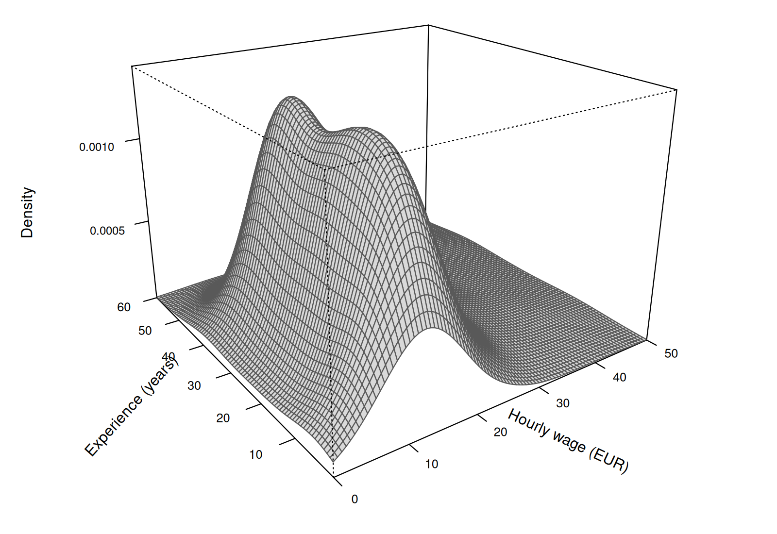
The joint density can be visualized as a surface over pairs of values.
(a) Joint density
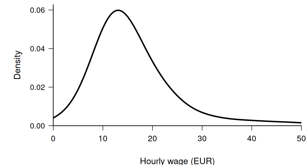
(b) Marginal density of wage
(c) Marginal density of experience
Figure 2.4: Joint and marginal densities of wage and experience
Integrating the surface over experience gives the marginal density of wage. Integrating over wage gives the marginal density of experience.
The marginal curves accumulate the surface along an axis. They are not slices at a fixed value.
Conditional Distributions
The conditional CDF of Y given Z=b is
F_{Y\mid Z=b}(a)=P(Y\leq a\mid Z=b).
It answers the question: If we know that Z=b, what is the distribution of Y?
If Z is discrete and P(Z=b)>0, the usual conditional-probability rule gives
F_{Y\mid Z=b}(a)
=\frac{P(Y\leq a,Z=b)}{P(Z=b)}.
\tag{2.1}
If both variables are discrete, the corresponding conditional PMF is
\pi_{Y\mid Z=b}(a)=\frac{\pi_{Y,Z}(a,b)}{\pi_Z(b)}.
If a joint density exists and f_Z(b)>0, the conditional density is
f_{Y\mid Z=b}(a)=\frac{f_{Y,Z}(a,b)}{f_Z(b)}.
\tag{2.2}
For a continuous Z, the event \{Z=b\} has probability zero. Therefore, the probability ratio in Equation 2.1 is not defined.
The density ratio in Equation 2.2 provides the corresponding conditional density.
Wage Given Education
Let Y denote wage and Z denote years of education.
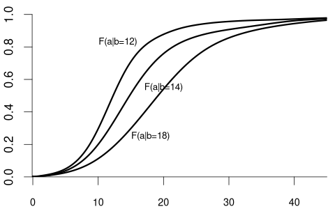
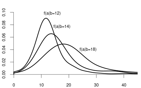
The conditional CDF F_{Y\mid Z=12}(a) describes the distribution of wages among individuals with 12 years of education.
(a) Conditional CDFs of wage given education
(b) Conditional PDFs of wage given education
Figure 2.5: Wage distributions conditional on education level
The plots show that the wage distribution varies with education.
At the threshold a=20,
P(Y\leq20\mid Z=12)>P(Y\leq20\mid Z=18).
Individuals with 12 years of education are more likely to have a wage no greater than 20 than individuals with 18 years of education.
This difference shows that wage and education are dependent random variables.
We can also condition on a random vector \boldsymbol X=(X_1,\ldots,X_k)':
F_{Y\mid\boldsymbol X=\boldsymbol x}(a)
=P(Y\leq a\mid\boldsymbol X=\boldsymbol x).
In the regression chapters, Y denotes the outcome and \boldsymbol X contains the regressors.
Recovering Marginal Distributions
A marginal distribution is a weighted average of conditional distributions.
If Z is discrete,
F_Y(a)=\sum_{b\in\mathcal Z}F_{Y\mid Z=b}(a)\pi_Z(b).
If Z has a density,
F_Y(a)=\int_{-\infty}^{\infty}F_{Y\mid Z=b}(a)f_Z(b)\,db.
These formulas are versions of the law of total probability.
2.5 Independence of Random Variables
The distribution of a coin flip should not depend on the marital status of the person tossing the coin.
In contrast, the wage distribution generally varies with education.
Independence
The random variables Y and Z are independent if and only if
F_{Y,Z}(a,b)=F_Y(a)F_Z(b)
for all a and b.
The definition has an equivalent and intuitive formulation:
F_{Y\mid Z=b}(a)=F_Y(a)
\tag{2.3} for all a.
In words, knowing the value of Z gives us no additional information about Y: the distribution of Y is the same whether or not we know Z=b.
For discrete Z, Equation 2.3 must hold for every b with P(Z=b)>0.
For continuous Z, Equation 2.3 must hold for almost all values of b. More precisely, there may be a set B of exceptional values such that P(Z\in B)=0, and the condition only needs to hold for b\notin B.
The conditional CDF of the coin flip is therefore the same for married and unmarried individuals.
If both Y and Z are discrete, independence is also equivalent to
\pi_{Y,Z}(a,b)=\pi_Y(a)\pi_Z(b)
for all a and b.
When a joint density exists, independence is equivalent to f_Y(a)f_Z(b) being a joint density of (Y,Z). Thus, we can write
f_{Y,Z}(a,b)=f_Y(a)f_Z(b).
For every b with f_Z(b)>0, the corresponding conditional density is
f_{Y\mid Z=b}(a)
=\frac{f_{Y,Z}(a,b)}{f_Z(b)}
=f_Y(a).
2.6 Expected Values
The expected value summarizes the center of a distribution.
More generally, we can take the expected value of a function h(Y).
An interval (a,b] receives the probability weight
F_Y(b)-F_Y(a)=P(a<Y\leq b).
If Y is discrete and the interval contains only one possible value u, this weight is the jump
\pi_Y(u)=P(Y=u).
If Y has a density, the probability weights can be written as
dF_Y(u)=f_Y(u)\,du.
The Stieltjes integral uses dF_Y(u) to cover both cases in one definition.
Expected Value
The expected value of h(Y) is
E[h(Y)]=\int_{-\infty}^{\infty}h(u)\,dF_Y(u),
provided that \int_{-\infty}^{\infty}|h(u)|\,dF_Y(u)<\infty.
If Y is discrete,
E[h(Y)]=\sum_{u\in\mathcal Y}h(u)\pi_Y(u).
If Y has a density,
E[h(Y)]=\int_{-\infty}^{\infty}h(u)f_Y(u)\,du.
For readers interested in the technical details of the Stieltjes integral, see Expected Value: General Case in my probability tutorial notes.
Taking h(u)=u gives the expected value E[Y], also called the population mean.
For a dummy variable Y, E[Y]=P(Y=1).
For the education distribution above, \begin{align*}
E[Y]
&=10(0.06)+12(0.43)+14(0.16) \\
&\quad+16(0.08)+18(0.24)+21(0.03) \\
&=14.23.
\end{align*}
Expectation is linear. For constants a,b,c,
E[a+bY+cZ]=a+bE[Y]+cE[Z].
This rule does not require Y and Z to be independent.
Expectations of random vectors and matrices are taken component by component.
2.7 Conditional Expectation
The conditional expectation is the mean of a conditional distribution.
Suppose that E[|Y|]<\infty. For values \boldsymbol x at which the conditional distribution is defined, let
m(\boldsymbol x)
:=E[Y\mid\boldsymbol X=\boldsymbol x]
=\int_{-\infty}^{\infty}y\,dF_{Y\mid\boldsymbol X=\boldsymbol x}(y).
The function m(\boldsymbol x) is called the conditional expectation function (CEF).
If Y is discrete,
E[Y\mid\boldsymbol X=\boldsymbol x]
=\sum_{y\in\mathcal Y}y\pi_{Y\mid\boldsymbol X=\boldsymbol x}(y).
If Y has a conditional density,
E[Y\mid\boldsymbol X=\boldsymbol x]
=\int_{-\infty}^{\infty}y f_{Y\mid\boldsymbol X=\boldsymbol x}(y)\,dy.
It is important to distinguish between:
E[Y\mid\boldsymbol X=\boldsymbol x]=m(\boldsymbol x): a number for a fixed value \boldsymbol x.
E[Y\mid\boldsymbol X]=m(\boldsymbol X): a function of \boldsymbol X and therefore a random variable.
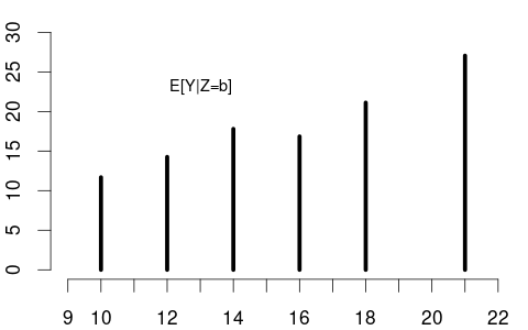
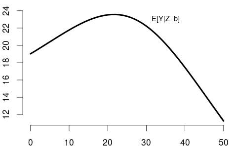
For wage Y and education Z, the CEF assigns a conditional mean wage to each education level:
m(b)=E[Y\mid Z=b].
(a) CEF of wage given education
(b) CEF of wage given experience
Figure 2.6: Conditional expectations of wage given education (left) and experience (right)
Rules for Conditional Expectations
The following rules hold whenever the expectations exist.
Conditional expectation is linear:
E[aA+bB\mid\boldsymbol X]
=aE[A\mid\boldsymbol X]+bE[B\mid\boldsymbol X].
Let r(\boldsymbol X) be a function of \boldsymbol X.
Once we condition on \boldsymbol X, the value of r(\boldsymbol X) is known. Therefore,
E[r(\boldsymbol X)\mid\boldsymbol X]=r(\boldsymbol X).
The conditioning theorem (CT), also called the factorization rule, states
E[r(\boldsymbol X)Y\mid\boldsymbol X]
=r(\boldsymbol X)E[Y\mid\boldsymbol X].
Thus, a function of \boldsymbol X can be taken outside the conditional expectation.
The law of iterated expectations (LIE) states
E[E[Y\mid\boldsymbol X]]=E[Y].
We can first calculate the mean within groups defined by \boldsymbol X, and then average these conditional means.
If Y and \boldsymbol X are independent, then
E[Y\mid\boldsymbol X]=E[Y].
The converse is not generally true. The equality E[Y\mid\boldsymbol X]=E[Y] means that Y is mean independent of \boldsymbol X, which is weaker than independence.
The CEF error is
u:=Y-m(\boldsymbol X).
This gives the exact decomposition
Y=m(\boldsymbol X)+u.
By construction, the CEF error has conditional mean zero: \begin{align*}
E[u\mid\boldsymbol X]
&=E[Y-m(\boldsymbol X)\mid\boldsymbol X] \\
&=E[Y\mid\boldsymbol X]-m(\boldsymbol X)=0.
\end{align*}
Together, the LIE and CT then imply \begin{align*}
E[r(\boldsymbol X)u]
&=E\!\left[E[r(\boldsymbol X)u\mid\boldsymbol X]\right] \\
&=E[r(\boldsymbol X)E[u\mid\boldsymbol X]]=0.
\end{align*}
The CEF m(\boldsymbol x) describes how the conditional population mean of Y varies with \boldsymbol x.
Regression models specify or approximate this function. Marginal effects describe how m(\boldsymbol x) changes when a regressor changes.
2.8 From Population Distributions to Sample Data
So far, F_Y, \pi_Y, f_Y, and the CEF have described a hypothetical population.
In practice, the population distribution is usually unknown. We observe a sample Y_1,\ldots,Y_n.
For a discrete variable, relative frequencies provide a sample counterpart of the population PMF:
\widehat\pi_Y(a)=\frac{n(a)}{n},
where n(a) is the number of observations equal to a.
For a continuous variable, a histogram divides the range of values into fixed intervals called bins. The area of each bar represents the relative frequency of observations in that bin.
A kernel density estimate (KDE) provides a smooth estimate of the population density. It can be understood as a smooth moving-window version of a histogram: nearby observations receive more weight than distant observations.
The weighting rule is called a kernel, while the bandwidth controls the width of the neighborhood and therefore the smoothness of the estimated density.
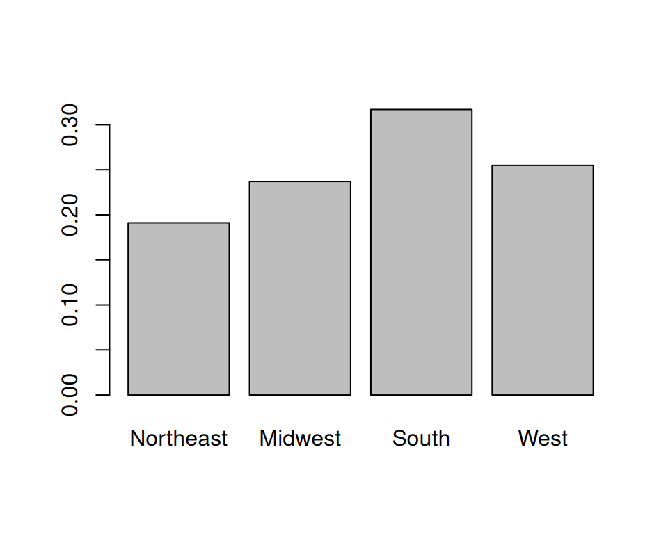
Let’s use the CPS data to estimate region probabilities and visualize the wage density:
cps=read.csv("cps.csv")n=length(cps$region)pmf=table(cps$region)/npar(mfrow =c(1, 2))barplot(pmf, names.arg =c("Northeast", "Midwest", "South", "West"), ylab ="Relative frequency", cex.names =0.75)hist(cps$wage, breaks =100, probability =TRUE, xlim =c(0, 80), xlab ="Hourly wage", ylab ="Density", main ="")lines(density(cps$wage, from =0, to =80), lwd =2)legend("topright", "KDE", lwd =2, bty ="n")
The bar plot shows relative frequencies for the four regions.
Across all bins, including wages above the displayed limit of 80, the areas sum to one.