5 Regression
5.1 Conditional Expectation
In econometrics, we often analyze how a variable of interest (like wages) varies systematically with other variables (like education or experience). The conditional expectation function (CEF) provides a powerful framework for describing these relationships.
The conditional expectation of a random variable Y given a random vector \boldsymbol X is the expected value of Y given any possible value of \boldsymbol X. Using the conditional CDF, the conditional expectation (or conditional mean) is E[Y|\boldsymbol X = \boldsymbol x] = \int_{-\infty}^\infty y \, dF_{Y|\boldsymbol X=\boldsymbol x}(y). For a continuous random variable Y we have E[Y|\boldsymbol X = \boldsymbol x] = \int_{-\infty}^\infty y \, f_{Y|\boldsymbol X = \boldsymbol x}(y) \, dy, where f_{Y|\boldsymbol X = \boldsymbol x}(y) is the conditional density of Y given \boldsymbol X = \boldsymbol x.
When Y is discrete with support \mathcal Y, we have E[Y|\boldsymbol X = \boldsymbol x] = \sum_{y \in \mathcal Y} y \, \pi_{Y|\boldsymbol X = \boldsymbol x}(y).
The CEF maps values of \boldsymbol X to corresponding conditional means of Y. As a function of the random vector \boldsymbol X, the CEF itself is a random variable: E[Y|\boldsymbol X] = m(\boldsymbol X), \quad \text{where } m(\boldsymbol x) = E[Y|\boldsymbol X = \boldsymbol x]
For a comprehensive treatment of conditional expectations see Probability Tutorial Part 2
Examples
Let’s examine this concept using wage and education as examples. When X is univariate and discrete (such as years of education), we can analyze how wage distributions change across education levels by comparing their conditional distributions:
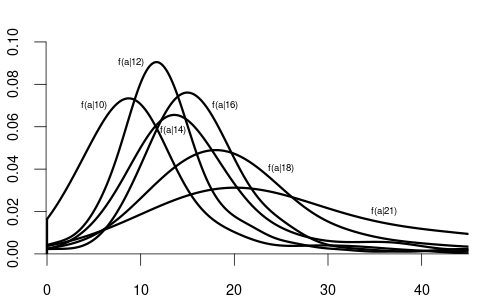
Notice how the conditional distributions tend to shift rightward as education increases, indicating higher average wages with higher education.
From these conditional densities, we can compute the expected wage for each education level. Plotting these conditional expectations gives the CEF: m(x) = E[\text{wage} \mid \text{edu} = x]
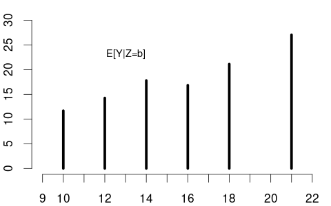
Since education is discrete, the CEF is defined only at specific values, as shown in the left plot below:
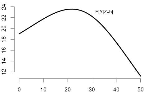
When X is continuous (like years of experience), the CEF is often a smooth function (right plot). The shape of E[\text{wage}|\text{experience}] reflects real-world patterns: wages rise quickly early in careers, then plateau, and may eventually decline near retirement.
The CEF as a Random Variable
It’s important to distinguish between:
- E[Y|\boldsymbol X = \boldsymbol x]: a number (the conditional mean at a specific value)
- E[Y|\boldsymbol X]: a function of \boldsymbol X, which is itself a random variable
For instance, if X = \text{education} has the probability mass function: P(X = x) = \begin{cases} 0.06 & \text{if } x = 10 \\ 0.43 & \text{if } x = 12 \\ 0.16 & \text{if } x = 14 \\ 0.08 & \text{if } x = 16 \\ 0.24 & \text{if } x = 18 \\ 0.03 & \text{if } x = 21 \\ 0 & \text{otherwise} \end{cases}
Then E[Y|X] as a random variable has the probability mass function: P(E[Y|X] = y) = \begin{cases} 0.06 & \text{if } y = 11.68 \text{ (when } X = 10\text{)} \\ 0.43 & \text{if } y = 14.26 \text{ (when } X = 12\text{)} \\ 0.16 & \text{if } y = 17.80 \text{ (when } X = 14\text{)} \\ 0.08 & \text{if } y = 16.84 \text{ (when } X = 16\text{)} \\ 0.24 & \text{if } y = 21.12 \text{ (when } X = 18\text{)} \\ 0.03 & \text{if } y = 27.05 \text{ (when } X = 21\text{)} \\ 0 & \text{otherwise}, \end{cases} where the values for y are taken from Figure 5.2 (a).
The CEF assigns to each value of \boldsymbol X the expected value of Y given that information.
5.2 CEF Properties
The conditional expectation function has several important properties that make it a fundamental tool in econometric analysis.
Law of Iterated Expectations (LIE)
The law of iterated expectations connects conditional and unconditional expectations: E[Y] = E[E[Y|\boldsymbol X]]
This means that to compute the overall average of Y, we can first compute the average of Y within each group defined by \boldsymbol X, then average those conditional means using the distribution of \boldsymbol X.
This is analogous to the law of total probability, where we compute marginal probabilities or densities as weighted averages of conditional ones:
For simplicity consider a univariate conditioning random variable X. When X is discrete: P(Y = y) = \sum_{x} P(Y = y \mid X = x) \cdot P(X = x)
When X is continuous: f_Y(y) = \int_{-\infty}^{\infty} f_{Y|X = x}(y) \cdot f_{X}(x) \, dx
Similarly, the LIE states:
When X is discrete: E[Y] = \sum_x E[Y \mid X = x] \cdot P(X = x)
When X is continuous: E[Y] = \int_{-\infty}^{\infty} E[Y \mid X = x] \cdot f_X(x) \, dx
Let’s apply this to our wage and education example. With X = \text{education} and Y = \text{wage}, we have:
\begin{aligned} E[Y|X=10] &= 11.68, \quad &P(X=10) = 0.06 \\ E[Y|X=12] &= 14.26, \quad &P(X=12) = 0.43 \\ E[Y|X=14] &= 17.80, \quad &P(X=14) = 0.16 \\ E[Y|X=16] &= 16.84, \quad &P(X=16) = 0.08 \\ E[Y|X=18] &= 21.12, \quad &P(X=18) = 0.24 \\ E[Y|X=21] &= 27.05, \quad &P(X=21) = 0.03 \end{aligned}
The law of iterated expectations gives us: \begin{aligned} E[Y] &= \sum_x E[Y|X = x] \cdot P(X = x) \\ &= 11.68 \cdot 0.06 + 14.26 \cdot 0.43 + 17.80 \cdot 0.16 \\ &\quad + 16.84 \cdot 0.08 + 21.12 \cdot 0.24 + 27.05 \cdot 0.03 \\ &= 0.7008 + 6.1318 + 2.848 + 1.3472 + 5.0688 + 0.8115 \\ &= 16.91 \end{aligned}
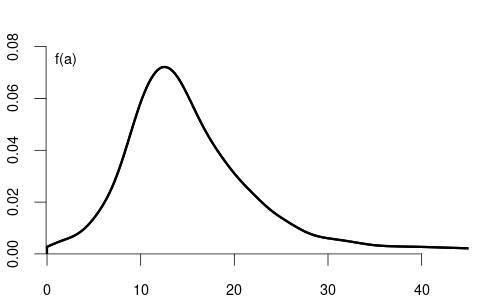
This unconditional expected wage of 16.91 aligns with what we would calculate from the unconditional density from Figure 5.1 (a).
The LIE provides us with a powerful way to bridge conditional expectations (within education groups) and the overall unconditional expectation (averaging across all education levels).
Conditioning Theorem (CT)
The conditioning theorem (also called the factorization rule) states: E[g(\boldsymbol X)Y | \boldsymbol X] = g(\boldsymbol X) \cdot E[Y | \boldsymbol X]
This means that when taking the conditional expectation of a product where one factor is a function of the conditioning variable, that factor can be treated as a constant and factored out. Once we condition on \boldsymbol X, the value of g(\boldsymbol X) is fixed.
If Y = \text{wage} and X = \text{education}, then for someone with 16 years of education: E[16 \cdot \text{wage} \mid \text{edu} = 16] = 16 \cdot E[\text{wage} \mid \text{edu} = 16]
More generally, if we want to find the expected product of education and wage, conditional on education: E[\text{edu} \cdot \text{wage} \mid \text{edu}] = \text{edu} \cdot E[\text{wage} \mid \text{edu}]
Best Predictor Property
If E[Y^2] < \infty, the conditional expectation E[Y|\boldsymbol X] is the best predictor of Y given \boldsymbol X in terms of mean squared error, i.e.: E[Y|\boldsymbol X] = \arg\min_{g(\cdot)} E[(Y - g(\boldsymbol X))^2]
This means that among all possible functions of \boldsymbol X, the CEF minimizes the expected squared prediction error. In practical terms, if you want to predict wages based only on education, the optimal prediction is exactly the conditional mean wage for each education level.
For example, if someone has 18 years of education, our best prediction of their wage (minimizing expected squared error) is E[\text{wage}|\text{education}=18] = 21.12.
No other function of education, whether linear, quadratic, or more complex, can yield a better prediction in terms of expected squared error than the CEF itself.
Proof sketch: Add and subtract m(\boldsymbol X) = E[Y|\boldsymbol X]: \begin{align*} &E[(Y-g(\boldsymbol X))^2] \\ &= E[(Y-m(\boldsymbol X) + m(\boldsymbol X) - g(\boldsymbol X))^2] \\ &= E[(Y-m(\boldsymbol X))^2] \\ &\quad + 2E[(Y-m(\boldsymbol X))(m(\boldsymbol X) - g(\boldsymbol X))] \\ &\quad + E[(m(\boldsymbol X) - g(\boldsymbol X))^2] \end{align*}
- The first term is finite and does not depend on g(\cdot).
- The cross term is zero by the LIE and CT.
- The last term is minimal if g(\boldsymbol X) = m(\boldsymbol X).
Independence Implications
If Y and \boldsymbol X are independent, then: E[Y|\boldsymbol X] = E[Y]
When variables are independent, knowing \boldsymbol X provides no information about Y, so the conditional expectation equals the unconditional expectation. The CEF becomes a constant function that doesn’t vary with \boldsymbol X.
In our wage example, if education and wage were completely independent, the CEF would be a horizontal line at the overall average wage of 16.91. Each conditional density f_{Y|\boldsymbol X = \boldsymbol x}(y) would be identical to the unconditional density f_Y(y), and the conditional means would all equal the unconditional mean.
The fact that our CEF for wage given education has a positive slope indicates that these variables are not independent – higher education is associated with higher expected wages.
5.3 Linear Model Specification
Prediction Error
Consider a sample (Y_i, \boldsymbol X_i'), i=1, \ldots, n. We have established that the conditional expectation function (CEF) E[Y_i|\boldsymbol X_i] is the best predictor of Y_i given \boldsymbol X_i, minimizing the mean squared prediction error.
This leads to the following prediction error: u_i = Y_i - E[Y_i|\boldsymbol X_i]
By construction, this error has a conditional mean of zero: E[u_i | \boldsymbol X_i] = 0
This property follows directly from the law of iterated expectations: \begin{align*} E[u_i | \boldsymbol X_i] &= E[Y_i - E[Y_i|\boldsymbol X_i] \mid \boldsymbol X_i] \\ &= E[Y_i | \boldsymbol X_i] - E[E[Y_i|\boldsymbol X_i] \mid \boldsymbol X_i] \\ &= E[Y_i | \boldsymbol X_i] - E[Y_i | \boldsymbol X_i] = 0 \end{align*}
We can thus always decompose the outcome as: Y_i = E[Y_i|\boldsymbol X_i] + u_i
where E[u_i|\boldsymbol X_i] = 0. This equation is not yet a regression model. It’s simply the decomposition of Y_i into its conditional expectation and an unpredictable component.
Linear Regression Model
To move to a regression framework, we impose a structural assumption about the form of the CEF. The key assumption of the linear regression model is that the conditional expectation is a linear function of the regressors: E[Y_i | \boldsymbol X_i] = \boldsymbol X_i'\boldsymbol \beta
Substituting this into our decomposition yields the linear regression equation: Y_i = \boldsymbol X_i'\boldsymbol \beta + u_i \tag{5.1}
with the crucial assumption: E[u_i | \boldsymbol X_i] = 0 \tag{5.2}
Exogeneity
This assumption (Equation 5.2) is called exogeneity or mean independence. It ensures that the linear function \boldsymbol X_i'\boldsymbol \beta correctly captures the conditional mean of Y_i.
Under the linear regression equation (Equation 5.1) we have the following equivalence: E[Y_i | \boldsymbol X_i] = \boldsymbol X_i'\boldsymbol \beta \quad \Leftrightarrow \quad E[u_i | \boldsymbol X_i] = 0
Therefore, the linear regression model in its most general form is characterized by the two conditions: linear regression equation (Equation 5.1) and exogenous regressors (Equation 5.2).
For example, in a wage regression, exogeneity means that the expected wage conditional on education and experience is exactly captured by the linear combination of these variables. No systematic pattern remains in the error term.
Model Misspecification
If the true conditional expectation function is nonlinear (e.g., if wages increase with education at a diminishing rate), then E[Y_i | \boldsymbol X_i] \neq \boldsymbol X_i'\boldsymbol \beta, and the model is misspecified. In such cases, the linear model provides the best linear approximation to the true CEF, but systematic patterns remain in the error term.
It’s important to note that u_i may still be statistically dependent on \boldsymbol X_i in ways other than its mean. For example, the variance of u_i may depend on \boldsymbol X_i in the case of heteroskedasticity. For instance, wage dispersion might increase with education level. The assumption E[u_i | \boldsymbol X_i] = 0 requires only that the conditional mean of the error is zero, not that the error is completely independent of the regressors.
5.4 Population Regression Coefficient
Under the linear regression model Y_i = \boldsymbol X_i'\boldsymbol \beta + u_i, \quad E[u_i | \boldsymbol X_i] = 0, we are interested in the population regression coefficient \boldsymbol \beta, which indicates how the conditional mean of Y_i varies linearly with the regressors in \boldsymbol X_i.
Moment Condition
A key implication of the exogeneity condition E[u_i | \boldsymbol X_i] = 0 is that the regressors are mean uncorrelated with the error term: E[\boldsymbol X_i u_i] = \boldsymbol 0
This can be derived from the exogeneity condition using the LIE: E[\boldsymbol X_i u_i] = E[E[\boldsymbol X_i u_i \mid \boldsymbol X_i]] = E[\boldsymbol X_i \cdot E[u_i | \boldsymbol X_i]] = E[\boldsymbol X_i \cdot 0] = \boldsymbol 0
Substituting the linear model into the mean uncorrelatedness condition gives a moment condition that identifies \boldsymbol \beta: \boldsymbol 0 = E[\boldsymbol X_i u_i] = E[\boldsymbol X_i (Y_i - \boldsymbol X_i'\boldsymbol \beta)] = E[\boldsymbol X_i Y_i] - E[\boldsymbol X_i \boldsymbol X_i']\boldsymbol \beta
Rearranging to solve for \boldsymbol \beta: E[\boldsymbol X_i Y_i] = E[\boldsymbol X_i \boldsymbol X_i'] \boldsymbol \beta
Assuming that the matrix E[\boldsymbol X_i \boldsymbol X_i'] is invertible, we can express the population regression coefficient as: \boldsymbol \beta = \left(E[\boldsymbol X_i \boldsymbol X_i']\right)^{-1} E[\boldsymbol X_i Y_i] \tag{5.3}
This expression shows that \boldsymbol \beta is entirely determined by the joint distribution of (Y_i, \boldsymbol X_i') in the population.
The invertibility of E[\boldsymbol X_i \boldsymbol X_i'] is guaranteed if there is no perfect linear relationship among the regressors. In particular, no pair of regressors should be perfectly correlated, and no regressor should be a perfect linear combination of the other regressors.
OLS Estimation
Recall that we have estimated population moments like E[Y] and \mathrm{Var}(Y) by their sample counterparts, i.e. \overline Y and \widehat \sigma_{Y}^2. This estimation principle is known as the method of moments, where we replace population moments by their corresponding sample moments.
To estimate the population regression coefficient \boldsymbol \beta = \left(E[\boldsymbol X_i \boldsymbol X_i']\right)^{-1} E[\boldsymbol X_i Y_i] using a given i.i.d. sample (Y_i, \boldsymbol X_i'), i=1, \ldots, n, we replace all population moments by their sample counterparts, i.e., \widehat{\boldsymbol \beta} = \left( \frac{1}{n} \sum_{i=1}^n \boldsymbol X_i \boldsymbol X_i' \right)^{-1} \left( \frac{1}{n} \sum_{i=1}^n \boldsymbol X_i Y_i \right).
This can be simplified to the familiar form \widehat{\boldsymbol \beta} = \left(\sum_{i=1}^n \boldsymbol X_i \boldsymbol X_i' \right)^{-1} \left(\sum_{i=1}^n \boldsymbol X_i Y_i \right), or \widehat{\boldsymbol \beta} = (\boldsymbol X'\boldsymbol X)^{-1}\boldsymbol X'\boldsymbol Y, which is called the ordinary least squares (OLS) estimator.
5.5 Consistency
Recall that the law of large numbers for a univariate i.i.d. dataset Y_1, \ldots, Y_n states that the sample average converges in probability to the population mean: \frac{1}{n} \sum_{i=1}^n Y_i \overset{p}{\to} E[Y] \quad \text{as } n \to \infty.
The OLS estimator is a function of two sample averages: the sample second moment matrix \frac{1}{n} \sum_{i=1}^n \boldsymbol{X}_i \boldsymbol{X}_i' and the sample cross-moment vector \frac{1}{n} \sum_{i=1}^n \boldsymbol{X}_i Y_i.
If (Y_i, \boldsymbol{X}_i'), i = 1, \ldots, n, are i.i.d., then the multivariate version of the law of large numbers applies:
\frac{1}{n} \sum_{i=1}^n \boldsymbol{X}_i \boldsymbol{X}_i' \overset{p}{\to} E[\boldsymbol{X}_i\boldsymbol{X}_i'], \quad
\frac{1}{n} \sum_{i=1}^n \boldsymbol{X}_i Y_i \overset{p}{\to} E[\boldsymbol{X}_i Y_i].
This means that convergence in probability holds componentwise. Each element of the sample moment matrix and vector converges to its corresponding population counterpart.
The continuous mapping theorem and Slutsky’s lemma enable us to extend these convergence results to more complex expressions.
- If f(\cdot) is a continuous function and V_n \overset{p}{\to} c, then f(V_n) \overset{p}{\to} f(c) (continuous mapping theorem).
- If V_n \overset{p}{\to} c and W_n \overset{p}{\to} d then V_n W_n \overset{p}{\to} cd (Slutsky’s lemma).
Since matrix inversion is a continuous function, the continuous mapping theorem implies: \bigg( \frac{1}{n} \sum_{i=1}^n \boldsymbol{X}_i \boldsymbol{X}_i' \bigg)^{-1} \overset{p}{\to} \big(E[\boldsymbol{X}_i \boldsymbol{X}_i']\big)^{-1}. Applying Slutsky’s lemma to combine the two convergence results yields: \begin{align*} \widehat{\boldsymbol \beta} &= \left( \frac{1}{n} \sum_{i=1}^n \boldsymbol X_i \boldsymbol X_i' \right)^{-1} \left( \frac{1}{n} \sum_{i=1}^n \boldsymbol X_i Y_i \right) \\ &\overset{p}{\to} \big(E[\boldsymbol{X}_i \boldsymbol{X}_i']\big)^{-1} E[\boldsymbol X_i Y_i] = \boldsymbol \beta. \end{align*}
This establishes the consistency of the OLS estimator. We used the following regularity conditions:
- Random sampling: (Y_i, \boldsymbol{X}_i') are i.i.d.
- Exogeneity (mean independence): E[u_i|\boldsymbol X_i] = 0.
- Finite second moments: E[X_{ij}^2] < \infty and E[Y_i^2] < \infty.
- Full rank: E[\boldsymbol{X}_i\boldsymbol{X}_i'] is positive definite (hence invertible).
Neither normality nor homoskedasticity is required for consistency. Heteroskedasticity is fully compatible with OLS consistency.
For any two random variables Y and Z, the Cauchy-Schwarz inequality states |E[YZ]| \leq \sqrt{E[Y^2] E[Z^2]}. Specifically, |E[X_{ik}X_{il}]| \leq \sqrt{E[X_{ik}^2] E[X_{il}^2]} and |E[X_{ik}Y_{i}]| \leq \sqrt{E[X_{ik}^2] E[Y_{i}^2]}.
Therefore, the finite second moment condition ensures that E[\boldsymbol{X}_i \boldsymbol{X}_i'] and E[\boldsymbol{X}_i Y_i] are finite. The full rank condition ensures that E[\boldsymbol{X}_i \boldsymbol{X}_i']^{-1} exists. Thus, the full rank and finite second moments conditions ensure that \boldsymbol{\beta} is well-defined.
The exogeneity condition is crucial for OLS consistency. Without it, the model is misspecified, Equation 5.3 does not hold, and the OLS estimator would converge to the best linear predictor, which is the \boldsymbol \beta^* that minimizes E[(Y_i - \boldsymbol X_i' \boldsymbol b)^2].
Just as with the univariate law of large numbers, the i.i.d. assumption can be relaxed to accommodate other sampling schemes. Under clustered sampling with independent clusters, OLS consistency holds if the number of clusters grows large relative to cluster size as n \to \infty. For time series data, (Y_i, \boldsymbol{X}_i') must be stationary, and observations (Y_i, \boldsymbol{X}_i') and (Y_{i-j}, \boldsymbol{X}_{i-j}') must become independent as j increases (strong mixing / weak dependence).