The term \boldsymbol X_i u_i is observation i’s moment contribution, also called its regression score.
The random part of Equation 8.1 is the sum of these scores.
For independent observations, covariances between different scores are zero.
Under dependence, these covariance terms generally matter.
All sandwich covariance estimators have the form
\widehat{\mathrm{Var}}
(\widehat{\boldsymbol\beta})
=
\left(\sum_i\boldsymbol X_i\boldsymbol X_i'\right)^{-1}
\widehat{\boldsymbol B}
\left(\sum_i\boldsymbol X_i\boldsymbol X_i'\right)^{-1}.
\tag{8.2}
The sampling structure determines the middle matrix \widehat{\boldsymbol B}:
HC estimators combine individual scores.
Cluster-robust estimators combine scores within each cluster.
HAC estimators combine scores at different time lags.
Selecting another covariance estimator changes standard errors, confidence intervals, and tests.
It does not change the OLS point estimates or repair an invalid population moment condition.
8.2 Clustered Observations
Suppose there are G clusters.
Cluster g contains observations j=1,\ldots,M_g, and
n=\sum_{g=1}^G M_g.
The regression model is
Y_{gj}=\boldsymbol X_{gj}'\boldsymbol\beta+u_{gj}.
\tag{8.3}
Observations may be dependent within a cluster. Different clusters are assumed to be independent.
For example, we may randomly select many schools and observe several students within each selected school.
Students from the same school may share teachers, facilities, and local conditions.
Cluster Scores
The score of cluster g is the sum of its observation-level scores:
\boldsymbol S_g
:=\sum_{j=1}^{M_g}\boldsymbol X_{gj}u_{gj}.
The scores of different clusters are independent. The terms inside one cluster score need not be independent.
If each observation-level moment is zero, linearity of expectations gives the cluster moment
E[\boldsymbol S_g]
=\sum_{j=1}^{M_g}E[\boldsymbol X_{gj}u_{gj}]
=\boldsymbol 0.
\tag{8.4}
The LLN and CLT are now applied across clusters rather than across individual observations.
NoteCluster asymptotics
Cluster-robust inference requires the number of independent clusters G to increase.
It also requires finite moments, an invertible design, and no cluster that dominates the sample.
Merely adding more observations to a fixed number of clusters does not provide the same justification.
Cluster-Robust Covariance Matrix
Let
\widehat{\boldsymbol S}_g
:=\sum_{j=1}^{M_g}
\boldsymbol X_{gj}\widehat u_{gj}
be the estimated cluster score.
The cluster meat is
\widehat{\boldsymbol B}_{CR0}
:=\sum_{g=1}^G
\widehat{\boldsymbol S}_g\widehat{\boldsymbol S}_g'.
Substituting \widehat{\boldsymbol B}_{CR0} for \widehat{\boldsymbol B} in Equation 8.2 gives \widehat{\mathrm{Var}}_{CR0}(\widehat{\boldsymbol\beta}).
The outer product \widehat{\boldsymbol S}_g\widehat{\boldsymbol S}_g' retains all score covariances within cluster g.
For routine applications, we use the finite-sample correction
\widehat{\mathrm{Var}}_{CR1}
(\widehat{\boldsymbol\beta})
:=
\frac{G}{G-1}\frac{n-1}{n-k}
\widehat{\mathrm{Var}}_{CR0}
(\widehat{\boldsymbol\beta}).
\tag{8.5}
Here, k is the rank of the complete regression design, including any estimated fixed-effect indicators.
Finite-sample cluster corrections vary somewhat across software. Equation 8.5 is the CR1 correction used here.
CR0 is the natural estimator for the derivation. CR1 is our practical default.
Cluster at the level at which observations may be dependent.
The relevant number for inference is the number of independent clusters, not merely the number of rows.
NoteFew clusters
CR1 is justified when the number of clusters is sufficiently large.
With few clusters, normal and \chi^2 approximations may be inaccurate.
Using a t_{G-1} reference distribution is a common adjustment for a single restriction, but it is not an exact general solution.
Specialized small-cluster methods may then be required.
8.3 Panel Data and Fixed Effects
A panel dataset observes the same units repeatedly.
Let i=1,\ldots,N index units and t=1,\ldots,T index periods.
Rows from the same unit form a natural cluster because shocks may remain related over time.
We treat units as independent across i while allowing dependence across t within each unit.
Panel data also allow us to compare a unit with itself at different dates.
Unit Fixed Effects
Let \boldsymbol Z_{it} contain regressors that vary over time.
The unit fixed-effects model is
Y_{it}
=\alpha_i+\boldsymbol Z_{it}'\boldsymbol\beta+u_{it}.
\tag{8.6}
The unit effect\alpha_i represents the combined additive contribution of observed and unobserved characteristics that remain constant over time.
It may be related to the regressors.
If \alpha_i is omitted, it becomes part of the regression error.
Pooled OLS then generally violates the population moment condition when \alpha_i is related to \boldsymbol Z_{it}.
For a balanced panel, define the unit averages
\overline Y_i:=\frac{1}{T}\sum_{t=1}^T Y_{it},
\qquad
\overline{\boldsymbol Z}_i
:=\frac{1}{T}\sum_{t=1}^T\boldsymbol Z_{it},
\qquad
\overline u_i:=\frac{1}{T}\sum_{t=1}^T u_{it}.
Subtracting these averages from Equation 8.6 gives
Y_{it}-\overline Y_i
=
(\boldsymbol Z_{it}-\overline{\boldsymbol Z}_i)'
\boldsymbol\beta
+(u_{it}-\overline u_i).
\tag{8.7}
The time-invariant effect \alpha_i disappears.
OLS applied to Equation 8.7 is the within estimator.
It gives the same slope estimates as OLS with unit indicators after applying the usual normalization.
Fixed-effects coefficients are identified by variation within the same unit over time.
A coefficient can only be identified if its regressor has sufficient within-unit variation after accounting for the other regressors.
The main population condition is strict exogeneity:
E[u_{it}\mid
\alpha_i,
\boldsymbol Z_{i1},\ldots,\boldsymbol Z_{iT}]
=0
\qquad\text{for every }t.
\tag{8.8}
The error in period t must have conditional mean zero given the unit effect and the regressors from every period.
In particular, a current shock must not determine future regressor values.
Time Effects
The model can also include a separate effect for each period:
Y_{it}
=\alpha_i+\lambda_t
+\boldsymbol Z_{it}'\boldsymbol\beta+u_{it}.
\tag{8.9}
The time effects\lambda_t account for common additive changes that affect all units in period t.
The slope is then estimated from within-unit variation after removing these common time changes.
NoteWhat fixed effects do not solve
Unit effects remove time-invariant differences between units, not time-varying omitted variables.
Time-invariant regressors cannot be estimated separately from unit effects.
Reverse causality remains possible.
Lagged outcomes generally require methods beyond the usual within estimator when T is fixed.
Fixed effects therefore do not create a causal interpretation by themselves.
Traffic Fatalities
The Fatalities data contain annual observations for 48 US states from 1982 to 1988.
The outcome is the number of traffic fatalities per 10,000 residents. The regressor is the tax on a case of beer.
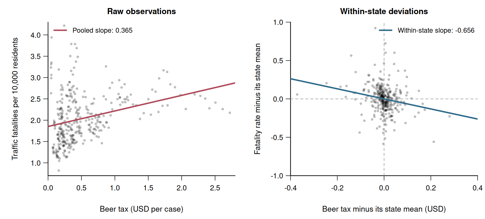
Figure 8.1: The pooled relationship combines differences across states and variation within states (left). Demeaning both variables by their state averages isolates within-state variation (right).
The pooled line slopes upward. The within-state line slopes downward.
This difference shows which comparisons determine the coefficient.
We estimate three specifications:
pooled OLS,
state fixed effects,
and state and year fixed effects.
Code
data("Fatalities", package ="AER")Fatalities$fatality_rate=10000*Fatalities$fatal/Fatalities$poppooled_fit=lm(fatality_rate~beertax, data =Fatalities)state_fe_fit=lm(fatality_rate~beertax+state, data =Fatalities)state_year_fe_fit=lm(fatality_rate~beertax+state+year, data =Fatalities)panel_models=list("Pooled"=pooled_fit,"State FE"=state_fe_fit,"State and year FE"=state_year_fe_fit)panel_vcov=lapply(panel_models,sandwich::vcovCL, cluster =Fatalities$state, type ="HC1")state_year_HC1=sandwich::vcovHC(state_year_fe_fit, type ="HC1")
With its cluster adjustment and type = "HC1", vcovCL() implements the CR1 correction in Equation 8.5.
The table reports standard errors clustered by state in parentheses.
Pooled
State FE
State and year FE
Beer tax
0.365
-0.656
-0.640
(0.120)
(0.315)
(0.386)
Num.Obs.
336
336
336
Adding state effects changes the point estimate because the coefficient is now estimated from within-state variation.
Adding year effects removes common additive changes shared by all states.
In the final specification, the estimated coefficient is -0.640.
The fitted model compares different years within the same state, after accounting for common year effects.
According to this model, years with a one-dollar higher beer tax have, on average, 0.640 fewer fatalities per 10,000 residents in that comparison.
Its HC1 standard error treating rows as independent is 0.255. The state-clustered standard error is 0.386.
The fixed effects change the fitted conditional-mean model. Clustering changes the estimated sampling uncertainty.
NoteDependence across two dimensions
State clustering allows arbitrary dependence over time within each state.
It does not allow remaining dependence between different states in the same year.
Time effects remove common changes in the conditional mean, but they need not remove all cross-state error dependence.
Two-way clustering by state and year can address both dimensions when there are many clusters in each dimension.
The seven years in this dataset are too few for reliable asymptotics based on year clusters.
8.4 Time Series
A time series observes variables in temporal order.
The index t is used because observations correspond to time points. T is the number of observed periods.
Nearby observations may be strongly related. We nevertheless need stable behavior as the sample period grows.
Stationarity
Let \boldsymbol W_t collect all variables observed in period t.
NoteStrict stationarity
The process \{\boldsymbol W_t\} is strictly stationary if
(\boldsymbol W_{t_1},\ldots,\boldsymbol W_{t_m})
\overset{d}{=}
(\boldsymbol W_{t_1+h},\ldots,\boldsymbol W_{t_m+h})
for every collection of dates and every admissible time shift h.
Thus, shifting the dates does not change their joint distribution.
If the second moments are finite, strict stationarity implies that
the mean and variance do not change over time,
and the covariance between two observations depends on their lag, not on their dates.
For a stationary scalar series with 0<\mathrm{Var}(Y_t)<\infty, the lag-h autocorrelation is
\rho(h)
:=\frac{\mathrm{Cov}(Y_t,Y_{t-h})}
{\mathrm{Var}(Y_t)}.
Stationarity concerns stability over time. It does not require observations to be independent.
Weak Dependence
A stationary process may still contain very persistent dependence.
For the LLN and CLT, dependence must become sufficiently weak as observations move farther apart in time.
We refer to this requirement as weak dependence.
The precise mathematical conditions differ across models. The central idea is that distant observations contain increasingly separate information.
Stationarity alone does not guarantee an LLN or CLT.
Time-series inference requires stationarity together with suitable weak dependence and moment conditions.
Stationary and Nonstationary Examples
The stationary solution of an AR(1) model satisfies
Y_t=\phi Y_{t-1}+\varepsilon_t,
\qquad |\phi|<1,
where the innovations \varepsilon_t are i.i.d. with mean zero and finite variance.
Its dependence declines geometrically: \rho(h)=\phi^{|h|}.
A random walk satisfies
Y_t=Y_{t-1}+\varepsilon_t.
\tag{8.10}
Here, the innovations \varepsilon_t are again i.i.d. with mean zero and finite variance.
Starting at Y_0=0 with innovation variance \sigma_\varepsilon^2,
\mathrm{Var}(Y_t)=t\sigma_\varepsilon^2.
Its distribution changes with t, so the random walk is nonstationary.
Its first difference
\Delta Y_t:=Y_t-Y_{t-1}=\varepsilon_t
is stationary.
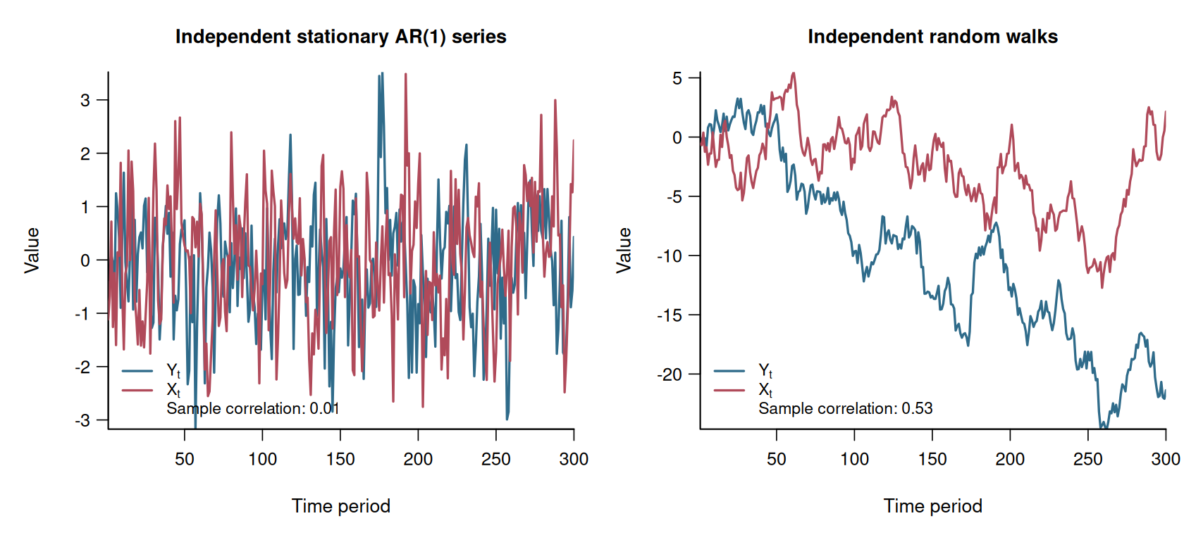
Figure 8.2: Two independently generated stable AR(1) processes do not show a persistent common path (left). Two independent random walks can move together for long periods purely by chance (right).
In this simulation, the sample correlation is 0.011 for the stationary series but 0.534 for the independent random walks.
After differencing the random walks, the sample correlation is -0.001.
Regressing unrelated nonstationary series on one another can produce a convincing but spurious regression.
HC, cluster-robust, and HAC standard errors do not solve this problem.
The conditional-mean condition implies the population moment
E[\boldsymbol X_tu_t]=\boldsymbol 0.
\tag{8.13}
If \boldsymbol Q is invertible, this moment identifies \boldsymbol\beta.
If only the moment holds, \boldsymbol\beta describes the best linear approximation rather than the exact CEF.
These conditions must follow from the economic question and timing of the variables. Dependence-robust standard errors cannot make them true.
Define
\boldsymbol S_t:=\boldsymbol X_tu_t.
The long-run covariance matrix of the scores is
\boldsymbol\Omega_{LR}
:=\sum_{h=-\infty}^{\infty}\boldsymbol\Gamma(h),
\qquad
\boldsymbol\Gamma(h)
:=E[\boldsymbol S_t\boldsymbol S_{t-h}'].
\tag{8.14}
It combines the contemporaneous score covariance with score covariances across all time lags.
NoteAsymptotic normality with time dependence
Suppose:
(Y_t,\boldsymbol X_t')' is stationary and sufficiently weakly dependent,
HC estimators retain only the contemporaneous term \boldsymbol\Gamma(0).
They are generally invalid when the regression scores remain correlated over time.
HAC Covariance Matrix
The Newey–West estimator combines estimated score covariances up to a selected maximum lag L.
It gives larger weights to short lags and gradually reduces the weights at longer lags.
Let \widehat{\boldsymbol\Omega}_{NW} denote the estimated long-run covariance defined below.
The HAC meat in Equation 8.2 is
\widehat{\boldsymbol B}_{HAC0}
:=T\widehat{\boldsymbol\Omega}_{NW}.
\tag{8.16}
Substituting this matrix into Equation 8.2 gives the natural HAC covariance estimator \widehat{\mathrm{Var}}_{HAC0}(\widehat{\boldsymbol\beta}).
For applications, we use the finite-sample adjustment
\widehat{\mathrm{Var}}_{HAC,adj}
(\widehat{\boldsymbol\beta})
:=\frac{T}{T-k}
\widehat{\mathrm{Var}}_{HAC0}
(\widehat{\boldsymbol\beta}).
\tag{8.17}
Here, T is the regression sample size and k is the number of estimated coefficients.
A small L may omit relevant dependence. A large L adds noisy long-lag covariance estimates.
NoteConstruction of the Newey–West estimator
Let
\widehat{\boldsymbol S}_t
:=\boldsymbol X_t\widehat u_t
be the estimated score.
For lag h\geq0, estimate its autocovariance by
\widehat{\boldsymbol\Gamma}(h)
:=\frac{1}{T}\sum_{t=h+1}^T
\widehat{\boldsymbol S}_t
\widehat{\boldsymbol S}_{t-h}'.
The Bartlett weight for lag h is
w_h:=1-\frac{h}{L+1}.
The Newey–West estimator of Equation 8.14 is
\widehat{\boldsymbol\Omega}_{NW}
:=\widehat{\boldsymbol\Gamma}(0)
+\sum_{h=1}^{L}w_h
\left[
\widehat{\boldsymbol\Gamma}(h)
+\widehat{\boldsymbol\Gamma}(h)'
\right].
For consistency, the maximum lag generally grows with the sample size but remains small relative to it:
L\to\infty
\qquad\text{and}\qquad
\frac{L}{T}\to0.
In applications, researchers use substantive knowledge, diagnostics, or an automatic rule to select L.
The lag choice should be reported.
Gasoline and Oil Returns
We use weekly gasoline and crude-oil prices from 1991 to 2023.
For a positive price P_t, its log return is
r_t:=\Delta\log(P_t)
=\log(P_t)-\log(P_{t-1}).
We first regress the current gasoline return on the first two lags of the oil return:
\mathrm{gas}_t
=\alpha+\delta_1\mathrm{oil}_{t-1}
+\delta_2\mathrm{oil}_{t-2}+u_t.
Under Equation 8.12, \delta_h compares weeks with different oil returns h weeks earlier and the same values of the other included lags.
It is the change in the mean gasoline return per unit difference in that lagged oil return.
The autoregressive distributed-lag specification additionally includes two lags of the gasoline return:
\mathrm{gas}_t
=\alpha+\delta_1\mathrm{oil}_{t-1}
+\delta_2\mathrm{oil}_{t-2}
+\phi_1\mathrm{gas}_{t-1}
+\phi_2\mathrm{gas}_{t-2}+u_t.
These outcome lags can represent persistence in gasoline returns.
If u_t remains serially correlated, however, \mathrm{gas}_{t-1} can be correlated with u_t because it contains earlier errors.
The population moment then fails, and HAC cannot repair it.
Code
data("gasoil", package ="teachingdata2")time_data=data.frame( date =gasoil$date[-1], gas =diff(log(gasoil$gasoline)), oil =diff(log(gasoil$brent)))time_data$gas_1=c(NA, head(time_data$gas, -1))time_data$gas_2=c(NA, NA, head(time_data$gas, -2))time_data$oil_1=c(NA, head(time_data$oil, -1))time_data$oil_2=c(NA, NA, head(time_data$oil, -2))DL_fit=lm(gas~oil_1+oil_2, data =time_data)ADL_fit=lm(gas~oil_1+oil_2+gas_1+gas_2, data =time_data)DL_HC1=sandwich::vcovHC(DL_fit, type ="HC1")DL_HAC=sandwich::NeweyWest(DL_fit, lag =12, prewhite =FALSE, adjust =TRUE)ADL_HAC=sandwich::NeweyWest(ADL_fit, lag =12, prewhite =FALSE, adjust =TRUE)
The HAC covariance matrices include score dependence up to 12 weeks.
The option adjust = TRUE applies the finite-sample factor in Equation 8.17.
This is an illustrative lag choice, not a universal default.
The table reports standard errors in parentheses.
DL: HC1
DL: HAC
ADL: HAC
Oil return, lag 1
0.171
0.171
0.124
(0.009)
(0.012)
(0.009)
Oil return, lag 2
0.085
0.085
0.008
(0.010)
(0.012)
(0.011)
Gasoline return, lag 1
0.375
(0.042)
Gasoline return, lag 2
0.109
(0.032)
Num.Obs.
1678
1678
1678
The two DL columns have identical point estimates.
For the first oil lag, the HC1 standard error is about 0.009 and the HAC standard error is about 0.012.
Adding outcome lags changes the conditional-mean specification and therefore the point estimates.
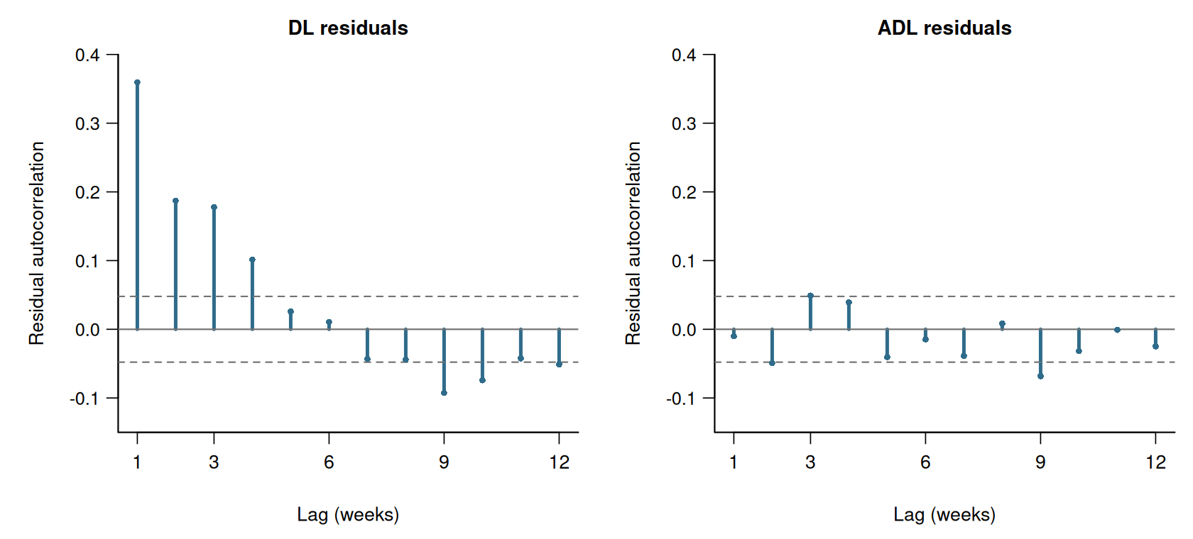
Figure 8.3: Sample autocorrelations of the residuals from the DL and ADL specifications. The dashed lines are rough 95% reference bounds under zero residual autocorrelation. The remaining lag-one autocorrelation is much smaller after adding the outcome lags.
The residual lag-one autocorrelation is 0.359 in the DL model and -0.010 in the ADL model.
The residual ACF is a useful diagnostic. It does not prove that all conditions for OLS or HAC inference hold.
HAC estimates uncertainty under stationary weak dependence.
It does not correct endogenous regressors, a poorly specified conditional mean, or nonstationary variables.
8.6 Inference with Dependent Observations
The confidence intervals and hypothesis tests from Sections 6 and 7 remain applicable.
We replace the HC1 covariance matrix by the estimator appropriate for the sampling structure.
Under H_0:\theta=\theta_0 and the corresponding large-sample conditions,
\frac{\widehat\theta-\theta_0}
{\mathrm{se}_{dep}(\widehat\theta)}
\overset{d}{\to}\mathcal N(0,1),
where \mathrm{se}_{dep} is based on CR1 or HAC.
The Wald test uses the corresponding covariance matrix in exactly the same way.
8.7 Dependent-Data Workflow
Identify which observations can reasonably be treated as independent.
Specify the conditional mean, including fixed effects or dynamics when required by the question.
Assess the moment condition and, for time series, stationarity and weak dependence.
Estimate the coefficient or effect of interest.
Select a covariance estimator that matches the sampling structure.
Report the number of clusters or time periods and any lag choices.
Interpret the population quantity without adding an unsupported causal claim.