(Intercept)   education      female
-14.081788 2.958174 -7.533067 7 Inference
7.1 Strict Exogeneity
Recall the linear regression framework:
- Regression equation Y_i = \boldsymbol{X}_i' \boldsymbol{\beta} + u_i, i=1, \ldots, n
- Exogeneity condition E[u_i | \boldsymbol{X}_i] = 0
- i.i.d. sample (Y_i, \boldsymbol{X}_i') with finite second moments
- Full rank E[\boldsymbol X_i \boldsymbol X_i']
The exogeneity condition
E[u_i | \boldsymbol{X}_i] = 0
ensures that the regressors are uncorrelated with the error at the individual observation level.
The i.i.d. condition implies (Y_i, \boldsymbol{X}_i') is independent of (Y_j, \boldsymbol{X}_j') for all j \neq i. Hence, \boldsymbol X_j is independent of u_i = Y_i - \boldsymbol X_i'\boldsymbol \beta for all j \neq i, so E[u_i | \boldsymbol X_1, \ldots, \boldsymbol X_n] = E[u_i | \boldsymbol{X}_i].
Together, exogeneity and i.i.d. sampling imply strict exogeneity: E[u_i | \boldsymbol X_1, \ldots, \boldsymbol X_n] = 0 \quad \text{for all} \ i. In cross-section with i.i.d. sampling, exogeneity at the unit level implies strict exogeneity.
Equivalently, in matrix form: E[\boldsymbol{u} | \boldsymbol{X}] = \boldsymbol{0}.
Strict exogeneity requires the entire vector of errors \boldsymbol{u} to be mean independent of the full regressor matrix \boldsymbol{X}. That is, no systematic relationship exists between any regressors and any error term across observations.
7.2 Unbiasedness
Under strict exogeneity, the OLS estimator \widehat{\boldsymbol{\beta}} is unbiased: E[\widehat{\boldsymbol{\beta}}] = \boldsymbol{\beta}.
Proof: Recall the model equation in matrix form: \boldsymbol{Y} = \boldsymbol{X}\boldsymbol{\beta} + \boldsymbol{u}.
Plugging this into the OLS formula: \begin{align*} \widehat{\boldsymbol{\beta}} &= (\boldsymbol{X}'\boldsymbol{X})^{-1} \boldsymbol{X}'\boldsymbol{Y} \\ &= (\boldsymbol{X}'\boldsymbol{X})^{-1} \boldsymbol{X}'(\boldsymbol{X} \boldsymbol{\beta} + \boldsymbol{u}) \\ &= \boldsymbol{\beta} + (\boldsymbol{X}'\boldsymbol{X})^{-1} \boldsymbol{X}'\boldsymbol{u}. \end{align*}
Taking the conditional expectation: E[\widehat{\boldsymbol{\beta}} | \boldsymbol{X}] = \boldsymbol{\beta} + (\boldsymbol{X}'\boldsymbol{X})^{-1} \boldsymbol{X}' E[\boldsymbol{u} | \boldsymbol{X}]. Since E[\boldsymbol u|\boldsymbol X] = \boldsymbol 0, the conditional mean is E[\widehat{\boldsymbol{\beta}} | \boldsymbol{X}] = \boldsymbol{\beta}. By the LIE, the unconditional mean becomes E[\widehat{\boldsymbol{\beta}}] = E[E[\widehat{\boldsymbol{\beta}} | \boldsymbol{X}]] = \boldsymbol{\beta}.
Thus, each element of the OLS estimator is unbiased: E[\widehat{\beta}_j] = \beta_j \quad \text{for } j = 1, \ldots, k.
7.3 Sampling Variance of OLS
The OLS estimator \widehat{\boldsymbol \beta} provides a point estimate of the unknown population parameter \boldsymbol \beta. For example, in the regression \text{wage}_i = \beta_1 + \beta_2 \text{education}_i + \beta_3 \text{female}_i + u_i, we obtain specific coefficient estimates:
The estimate for education is \widehat \beta_2 = 2.958. However, this point estimate tells us nothing about how far it might be from the true value \beta_2.
That is, it does not reflect estimation uncertainty, which arises because \widehat{\boldsymbol \beta} depends on a finite sample that could have turned out differently if a different dataset from the same population had been used.
Larger samples tend to reduce estimation uncertainty, but in practice we only observe one finite sample. To quantify this uncertainty, we study the sampling variance of the OLS estimator: \mathrm{Var}(\widehat{\boldsymbol \beta} | \boldsymbol X_1, \ldots, \boldsymbol X_n) = \mathrm{Var}(\widehat{\boldsymbol \beta} | \boldsymbol X), the conditional variance of \widehat{\boldsymbol \beta} given the regressors \boldsymbol X_1, \ldots, \boldsymbol X_n.
Sampling variance of OLS:
Under i.i.d. sampling, the OLS covariance matrix is \mathrm{Var}(\widehat{ \boldsymbol \beta} | \boldsymbol X) = \bigg( \sum_{i=1}^n \boldsymbol X_i \boldsymbol X_i' \bigg)^{-1} \sum_{i=1}^n \sigma_i^2 \boldsymbol X_i \boldsymbol X_i' \bigg( \sum_{i=1}^n \boldsymbol X_i \boldsymbol X_i' \bigg)^{-1}, where \sigma_i^2 = E[u_i^2 | \boldsymbol X_i].
In matrix notation, this can be equivalently written as \mathrm{Var}(\widehat{ \boldsymbol \beta} | \boldsymbol X) = (\boldsymbol X'\boldsymbol X)^{-1} \boldsymbol X' \mathrm{Var}(\boldsymbol u | \boldsymbol X) \boldsymbol X (\boldsymbol X'\boldsymbol X)^{-1}.
Proof: Recall the general rule that for any matrix \boldsymbol A, \mathrm{Var}(\boldsymbol A \boldsymbol u) = \boldsymbol A \, \mathrm{Var}(\boldsymbol u) \, \boldsymbol A'. Hence, with \boldsymbol A = (\boldsymbol X'\boldsymbol X)^{-1} \boldsymbol X', by the symmetry of (\boldsymbol X'\boldsymbol X)^{-1}, \begin{align*} \mathrm{Var}(\widehat{ \boldsymbol \beta} | \boldsymbol X) &= \mathrm{Var}(\boldsymbol \beta + (\boldsymbol X'\boldsymbol X)^{-1} \boldsymbol X' \boldsymbol u | \boldsymbol X) \\ &=\mathrm{Var}((\boldsymbol X'\boldsymbol X)^{-1} \boldsymbol X'\boldsymbol u|\boldsymbol X) \\ &= (\boldsymbol X'\boldsymbol X)^{-1} \boldsymbol X' \mathrm{Var}(\boldsymbol u | \boldsymbol X) ((\boldsymbol X'\boldsymbol X)^{-1} \boldsymbol X')' \\ &= (\boldsymbol X'\boldsymbol X)^{-1} \boldsymbol X' \mathrm{Var}(\boldsymbol u | \boldsymbol X) \boldsymbol X (\boldsymbol X'\boldsymbol X)^{-1}. \end{align*}
Under i.i.d. sampling, conditional on \boldsymbol X, u_i and u_j are independent for i \neq j, so E[u_i u_j|\boldsymbol X] = E[u_i|\boldsymbol X] \, E[u_j|\boldsymbol X] = E[u_i|\boldsymbol X_i] \, E[u_j|\boldsymbol X_j] = 0, and the conditional covariance matrix of \boldsymbol u takes a diagonal form: \mathrm{Var}(\boldsymbol u | \boldsymbol X) = \begin{pmatrix} \sigma_1^2 & 0 & \cdots & 0 \\ 0 & \sigma_2^2 & \cdots & 0 \\ \vdots & \vdots & \ddots & \vdots \\ 0 & 0 & \cdots & \sigma_n^2 \end{pmatrix}. Also note: \boldsymbol X' \mathrm{Var}(\boldsymbol u | \boldsymbol X) \boldsymbol X = \sum_{i=1}^n \sigma_i^2 \boldsymbol X_i \boldsymbol X_i' and \boldsymbol X'\boldsymbol X = \sum_{i=1}^n \boldsymbol X_i \boldsymbol X_i'.
Homoskedasticity
While u_i is uncorrelated with \boldsymbol X_i under the exogeneity assumption, its variance may depend on \boldsymbol X_i. We say that the errors are heteroskedastic: \sigma_i^2 = \mathrm{Var}(u_i | \boldsymbol X_i) = \sigma^2(\boldsymbol X_i).
In the specific situation where the conditional variance of the error does not depend on \boldsymbol X_i and is equal to \sigma^2 for any value of \boldsymbol X_i, we say that the errors are homoskedastic: \sigma^2 = \mathrm{Var}(u_i) = \mathrm{Var}(u_i | \boldsymbol X_i) \quad \text{for all} \ i.
The homoskedastic error covariance matrix has the following simple form: \mathrm{Var}(\boldsymbol u | \boldsymbol X) = \begin{pmatrix} \sigma^2 & 0 & \cdots & 0 \\ 0 & \sigma^2 & \cdots & 0 \\ \vdots & \vdots & \ddots & \vdots \\ 0 & 0 & \cdots & \sigma^2 \end{pmatrix} = \sigma^2 \boldsymbol{I}_n. Because \boldsymbol X' \mathrm{Var}(\boldsymbol u | \boldsymbol X) \boldsymbol X = \sigma^2 \boldsymbol X'\boldsymbol X, the resulting OLS covariance matrix reduces to \mathrm{Var}(\widehat{ \boldsymbol \beta} | \boldsymbol X) = \sigma^2 (\boldsymbol X'\boldsymbol X)^{-1} = \sigma^2 \bigg( \sum_{i=1}^n \boldsymbol X_i \boldsymbol X_i' \bigg)^{-1}.
7.4 Gaussian distribution
Univariate Normal distribution
The Gaussian distribution, also known as the normal distribution, is a fundamental concept in statistics.
A random variable Z is said to follow a normal distribution if it has the following probability density function (PDF): f_Z(z) = \frac{1}{\sqrt{2 \pi \sigma^2}} \exp\Big(-\frac{(z-\mu)^2}{2 \sigma^2}\Big). Formally, we denote this as Z \sim \mathcal N(\mu, \sigma^2), meaning that Z is normally distributed with mean \mu and variance \sigma^2.
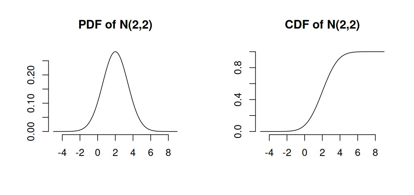
The normal distribution with mean 0 and variance 1 is called the standard normal distribution. It has the PDF \phi(u) = \frac{1}{\sqrt{2 \pi}} \exp\Big(-\frac{u^2}{2}\Big) and its CDF is \Phi(a) = \int_{-\infty}^a \phi(u) \, du. \mathcal N(0,1) is symmetric around zero: \phi(u) = \phi(-u), \quad \Phi(a) = 1 - \Phi(-a).
Standardizing: If Z \sim \mathcal N(\mu, \sigma^2), then \frac{Z-\mu}{\sigma} \sim \mathcal N(0,1). The CDF of Z is P(Z \leq a) = \Phi((a-\mu)/\sigma).
A normally distributed random variable Z has \mathrm{skew}(Z) = 0 and \mathrm{kurt}(Z) = 3.
Linear combinations of normally distributed variables are normal: If Y_1, \ldots, Y_n are jointly normally distributed and c_1, \ldots, c_n \in \mathbb R, then \sum_{j=1}^n c_j Y_j is normally distributed.
Multivariate Normal distribution
Let Z_1, \ldots, Z_k be independent \mathcal N(0,1) random variables.
Then, the k-vector \boldsymbol Z = (Z_1, \ldots, Z_k)' has the multivariate standard normal distribution, written \boldsymbol Z \sim \mathcal N(\boldsymbol 0, \boldsymbol I_k). Its joint PDF is f(\boldsymbol x) = \frac{1}{(2 \pi)^{k/2}} \exp\left( - \frac{\boldsymbol x'\boldsymbol x}{2} \right).
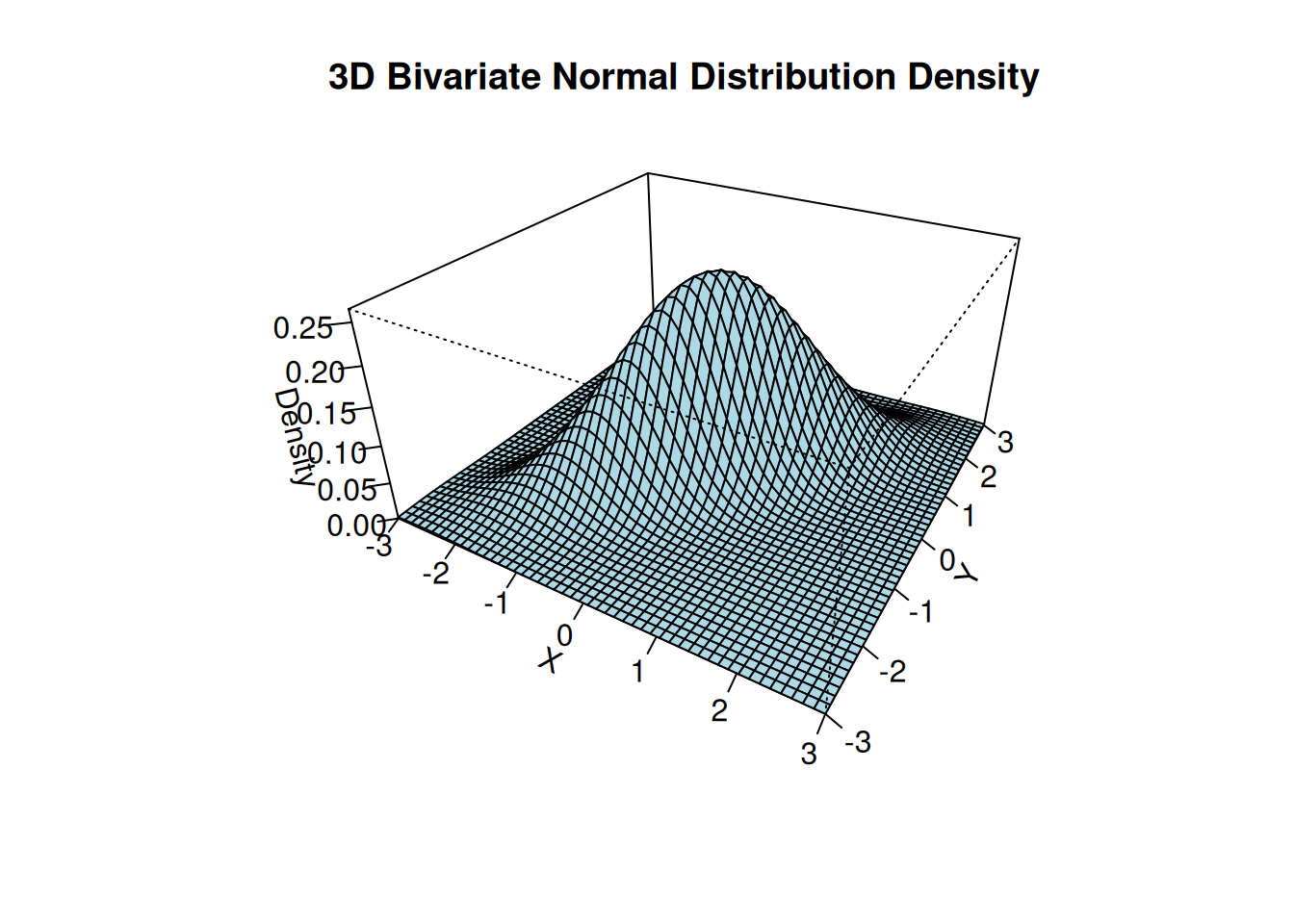
If \boldsymbol Z \sim \mathcal N(\boldsymbol 0, \boldsymbol I_k) and \boldsymbol Z^* = \boldsymbol \mu + \boldsymbol B \boldsymbol Z for a q \times 1 vector \boldsymbol \mu and a q \times k matrix \boldsymbol B, then \boldsymbol Z^* has a multivariate normal distribution with mean vector \boldsymbol \mu and covariance matrix \boldsymbol \Sigma = \boldsymbol B \boldsymbol B', written \boldsymbol Z^* \sim \mathcal N(\boldsymbol \mu, \boldsymbol \Sigma).
The q-variate PDF of \boldsymbol Z^* is f(\boldsymbol u) = \frac{1}{(2 \pi)^{q/2} (\det(\boldsymbol \Sigma))^{1/2} } \exp\Big(- \frac{1}{2}(\boldsymbol u-\boldsymbol \mu)'\boldsymbol \Sigma^{-1} (\boldsymbol u-\boldsymbol\mu) \Big).
The mean vector and covariance matrix are E[\boldsymbol Z^*] = \boldsymbol \mu, \quad \mathrm{Var}(\boldsymbol Z^*) = \boldsymbol \Sigma.
The 3D plot below shows the bivariate normal PDF with parameters \boldsymbol \mu = \begin{pmatrix} 0 \\ 0 \end{pmatrix}, \quad \boldsymbol \Sigma = \begin{pmatrix} 1 & 0.8 \\ 0.8 & 1 \end{pmatrix}.
7.5 Gaussian Regression Model
The Gaussian regression model builds on the linear regression framework by adding a distributional assumption in addition to the i.i.d. and exogeneity assumptions.
It assumes that the error terms are homoskedastic and conditionally normally distributed: u_i | \boldsymbol{X}_i \sim \mathcal{N}(0, \sigma^2) \tag{7.1}
That is, conditional on the regressors, the error has mean zero (exogeneity), constant variance (homoskedasticity), and a normal distribution.
Because u_i = Y_i - \boldsymbol X_i'\boldsymbol \beta, Equation 7.1 is equivalent to Y_i|\boldsymbol X_i \sim \mathcal N( \boldsymbol X_i'\boldsymbol \beta, \sigma^2). Thus, the normality assumption is a distributional assumption about the dependent variable Y_i, not the regressors \boldsymbol X_i.
Because \widehat{\boldsymbol \beta} is a linear combination of the independent and normally distributed variables Y_1, \ldots, Y_n, the OLS estimator is also normally distributed: \widehat{\boldsymbol{\beta}} | \boldsymbol{X} \sim \mathcal{N}\Big(\boldsymbol{\beta}, \mathrm{Var}(\widehat{ \boldsymbol \beta} | \boldsymbol X)\Big).
The variance of the j-th OLS coefficient \widehat \beta_j is the j-th diagonal element of the covariance matrix. Under homoskedasticity, its conditional standard deviation is \mathrm{sd}(\widehat \beta_j | \boldsymbol X) = \sqrt{ \big(\mathrm{Var}(\widehat{ \boldsymbol \beta} | \boldsymbol X) \big)_{jj}} = \sigma \sqrt{\big((\boldsymbol{X}'\boldsymbol{X})^{-1}\big)_{jj}}.
Subtracting the mean E[\widehat \beta_j] = \beta_j and dividing by the \mathrm{sd}(\widehat{ \boldsymbol \beta} | \boldsymbol X) gives the standardized OLS coefficient, which has mean zero and variance 1: Z_j := \frac{\widehat \beta_j - \beta_j}{\mathrm{sd}(\widehat \beta_j | \boldsymbol X)} \sim \mathcal N(0,1)
7.6 Classical Standard Errors
The conditional standard deviation \mathrm{sd}(\widehat \beta_j | \boldsymbol X) in the Gaussian regression model is unknown because the population error variance \sigma^2 is unknown: \mathrm{sd}(\widehat \beta_j | \boldsymbol X) = \sigma \sqrt{\big((\boldsymbol{X}'\boldsymbol{X})^{-1}\big)_{jj}}.
A standard error of \widehat \beta_j is an estimator of the conditional standard deviation. To construct a valid standard error under this setup, we can use the adjusted residual variance to estimate \sigma^2: s_{\widehat{u}}^2 = \frac{1}{n-k} \sum_{i=1}^n \widehat{u}_i^2. The classical standard error (valid under homoskedasticity) is defined as: \mathrm{se}_{hom}(\widehat{\beta}_j) = s_{\widehat{u}} \sqrt{(\boldsymbol{X}'\boldsymbol{X})^{-1}_{jj}}.
To estimate the full sampling covariance matrix \boldsymbol V = \mathrm{Var}(\widehat{\boldsymbol \beta} \mid \boldsymbol X), the classical covariance matrix estimator is: \widehat{\boldsymbol V}_{hom} = s_{\widehat u}^2 (\boldsymbol X'\boldsymbol X)^{-1}.
## classical homoskedastic covariance matrix estimator:
vcov(fit)
(Intercept) education female
(Intercept) 0.18825476 -0.0127486354 -0.0089269796
education -0.01274864 0.0009225111 -0.0002278021
female -0.00892698 -0.0002278021 0.0284200217Classical standard errors \mathrm{se}_{hom}(\widehat{\beta}_j) are the square roots of the diagonal entries:
(Intercept)   education      female
 0.43388334  0.03037287  0.16858239
They are also displayed in parentheses in a typical regression summary table:
library(modelsummary)
modelsummary(fit, gof_map = "none")| (1) | |
|---|---|
| (Intercept) | -14.082 |
| (0.434) | |
| education | 2.958 |
| (0.030) | |
| female | -7.533 |
| (0.169) |
7.7 Distributions from Normal Samples
Chi-squared distribution
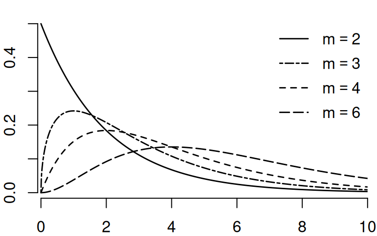
Let Z_1, \ldots, Z_m be independent \mathcal N(0,1) random variables. Then, the random variable Y = \sum_{i=1}^m Z_i^2 is chi-squared distributed with parameter m, written Y \sim \chi^2_{m}.
The parameter m is called the degrees of freedom.
Under the Gaussian assumption Equation 7.1, s_{\widehat{u}}^2 has the following property: \frac{(n-k) s_{\widehat{u}}^2}{\sigma^2} \sim \chi^2_{n-k}. \tag{7.2}
Student t-distribution
If Z \sim \mathcal N(0,1) and Q \sim \chi^2_{m}, and Z and Q are independent, then Y = \frac{Z}{\sqrt{Q/m}} is t-distributed with m degrees of freedom, written Y \sim t_m.
Under the Gaussian assumption Equation 7.1, the standardized OLS coefficient is standard normal.
When we replace the population standard deviation with its sample estimate (the standard error) then the standardized OLS coefficient has a t-distribution: T_j := \frac{\widehat \beta_j - \beta_j}{\mathrm{se}_{hom}(\widehat \beta_j)} = \frac{\widehat \beta_j - \beta_j}{\mathrm{sd}(\widehat \beta_j | \boldsymbol X)} \cdot \frac{\sigma}{s_{\widehat{u}}} = Z_j \cdot \frac{\sigma}{s_{\widehat{u}}} with T_j \sim \frac{\mathcal{N}(0,1)}{\sqrt{\chi^2_{n-k}/(n-k)}} = t_{n-k}. \tag{7.3} This means that the OLS coefficient standardized with the homoskedastic standard error instead of the standard deviation follows a t-distribution with n-k degrees of freedom.
Here, we used Equation 7.2 and the fact \widehat{\boldsymbol{\beta}} and s_{\widehat{u}}^2 are independent.
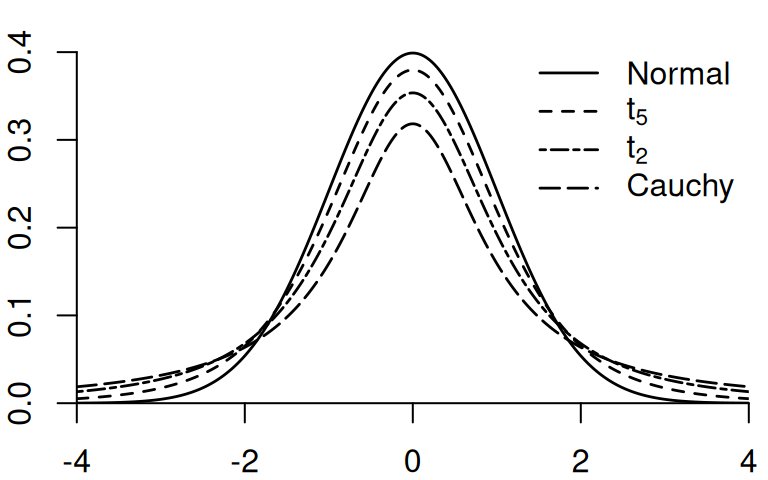
Like \mathcal N(0,1), the t-distribution is symmetric around zero: P(T_j > a) = P(T_j < -a).
The t-distribution has heavier tails than the standard normal distribution.
The t_m distribution approaches \mathcal N(0,1) as m \to \infty.
7.8 Exact Confidence Intervals
A confidence interval is a range of values that is likely to contain the true population parameter with a specified confidence level or coverage probability, often expressed as a percentage (e.g., 95%).
A (1 - \alpha) confidence interval for \beta_j is an interval I_{1-\alpha} such that P(\beta_j \in I_{1-\alpha}) = 1 - \alpha, \tag{7.4} or, equivalently, P(\beta_j \notin I_{1-\alpha}) = \alpha.
To construct such an interval, we use the form I_{1-\alpha} = \Big[ \widehat{\beta}_j - q \cdot \mathrm{se}_{hom}(\widehat{\beta}_j); \widehat{\beta}_j + q \cdot \mathrm{se}_{hom}(\widehat{\beta}_j) \Big]. To find the suitable value q, note that, by Equation 7.3, \begin{align*} P(\beta_j \in I_{1-\alpha}) &= P\Big( \widehat{\beta}_j - q \cdot \mathrm{se}_{hom}(\widehat{\beta}_j) \leq \beta_j \leq \widehat{\beta}_j + q \cdot \mathrm{se}_{hom}(\widehat{\beta}_j) \Big) \\ &= P\Big(- q \cdot \mathrm{se}_{hom}(\widehat{\beta}_j) \leq \beta_j - \widehat{\beta}_j \leq q \cdot \mathrm{se}_{hom}(\widehat{\beta}_j) \Big) \\ &= P\Big(- q \cdot \mathrm{se}_{hom}(\widehat{\beta}_j) \leq \widehat{\beta}_j - \beta_j \leq q \cdot \mathrm{se}_{hom}(\widehat{\beta}_j) \Big) \\ &=P\Big(- q \leq \frac{\widehat{\beta}_j - \beta_j}{\mathrm{se}_{hom}(\widehat{\beta}_j)} \leq q \Big) \\ &= P(|T_j| \leq q), \end{align*} or, equivalently, P(\beta_j \notin I_{1-\alpha}) = P(|T_j| > q). By the symmetry of the t-distribution, P(|T_j| > q) = P(T_j > q) + P(T_j < -q) = 2 P(T_j > q). Therefore, Equation 7.4 is equivalent to \begin{align*} &\phantom{\Leftrightarrow} \quad P(\beta_j \notin I_{1-\alpha}) = \alpha \\ &\Leftrightarrow \quad P(|T_j| > q) = \alpha \\ &\Leftrightarrow \quad 2 P(T_j > q) = \alpha \\ &\Leftrightarrow \quad P(T_j > q) = \alpha/2 \\ &\Leftrightarrow \quad P(T_j \leq q) = 1-\alpha/2. \end{align*} The last condition means that q must be the 1-\alpha/2 quantile of the distribution of T_j, which is the t_{n-k}-distribution.
We write q = t_{n-k, 1-\alpha/2}.
Hence, under the Gaussian regression model, P\bigg( \beta_j \in \Big[ \widehat{\beta}_j - t_{n-k, 1-\alpha/2} \cdot \mathrm{se}_{hom}(\widehat{\beta}_j); \widehat{\beta}_j + t_{n-k, 1-\alpha/2} \cdot \mathrm{se}_{hom}(\widehat{\beta}_j) \Big] \bigg) = 1-\alpha.
| df | 0.95 | 0.975 | 0.995 | 0.9995 |
|---|---|---|---|---|
| 1 | 6.31 | 12.71 | 63.66 | 636.6 |
| 2 | 2.92 | 4.30 | 9.92 | 31.6 |
| 3 | 2.35 | 3.18 | 5.84 | 12.9 |
| 5 | 2.02 | 2.57 | 4.03 | 6.87 |
| 10 | 1.81 | 2.23 | 3.17 | 4.95 |
| 20 | 1.72 | 2.09 | 2.85 | 3.85 |
| 50 | 1.68 | 2.01 | 2.68 | 3.50 |
| 100 | 1.66 | 1.98 | 2.63 | 3.39 |
| \to \infty | 1.64 | 1.96 | 2.58 | 3.29 |
The last row (indicated by \to \infty) shows the quantiles of the standard normal distribution \mathcal N(0,1).
You can display 95% confidence intervals in the modelsummary output using the conf.int argument:
modelsummary(fit, gof_map = "none", statistic = "conf.int")| (1) | |
|---|---|
| (Intercept) | -14.082 |
| [-14.932, -13.231] | |
| education | 2.958 |
| [2.899, 3.018] | |
| female | -7.533 |
| [-7.863, -7.203] |
7.9 Confidence Interval Interpretation
Note: the confidence interval is random, while the parameter \beta_j is fixed but unknown.

A correct interpretation of a 95% confidence interval is:
- If we were to repeatedly draw samples and construct a 95% confidence interval from each sample, about 95% of these intervals would contain the true parameter.
Common misinterpretations to avoid:
- ❌ “The true value has a 95% probability of being in this interval.”
- ❌ “We are 95% confident this interval contains the true parameter.”
These mistakes incorrectly treat the parameter as random and the interval as fixed. In reality, it’s the other way around.
A 95% confidence interval should be understood as a coverage probability: Before observing the data, there is a 95% probability that the random interval will cover the true parameter.
A helpful visualization:7.10 Limitations of the Gaussian Approach
The Gaussian regression framework assumes:
- Exogeneity: E[u_i \mid \boldsymbol X_i] = 0
- i.i.d. sample: (Y_i, \boldsymbol X_i'), i=1, \ldots, n
- Homoskedastic, normally distributed errors: u_i|\boldsymbol X_i \sim \mathcal{N}(0, \sigma^2)
- Full rank E[\boldsymbol X_i \boldsymbol X_i']
While mathematically convenient, these assumptions are often violated in practice. In particular, the normality assumption implies homoskedasticity and that the conditional distribution of Y_i given \boldsymbol X_i is normal, which is an unrealistic scenario in many economic applications.
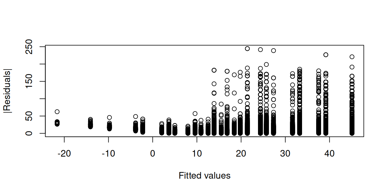
Historically, homoskedasticity has been treated as the “default” assumption and heteroskedasticity as a special case. But in empirical work, heteroskedasticity is the norm.
A plot of the absolute value of the residuals against the fitted values shows that individuals with predicted wages around 10 USD exhibit residuals with lower variance compared to those with higher predicted wage levels. Hence, the homoskedasticity assumption is implausible:
The Q-Q-plot is a graphical tool to help us assess if the errors are conditionally normally distributed.
Let \widehat u_{(i)} be the sorted residuals (i.e. \widehat u_{(1)} \leq \ldots \leq \widehat u_{(n)}). The Q-Q-plot plots the sorted residuals \widehat u_{(i)} against the ((i-0.5)/n)-quantiles of the standard normal distribution.
If the residuals line up well on the straight dashed line, there is an indication that the distribution of the residuals is close to a normal distribution.
set.seed(123)
par(mfrow = c(1,2))
## auxiliary regression with simulated normal errors:
fit.aux = lm(rnorm(500) ~ 1)
## Q-Q-plot of the residuals of the auxiliary regression:
qqnorm(residuals(fit.aux))
qqline(residuals(fit.aux))
## Q-Q-plot of the residuals of the wage regression:
qqnorm(residuals(fit))
qqline(residuals(fit))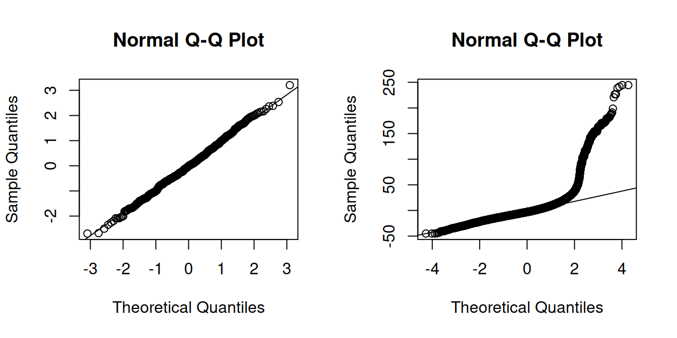
In the left plot you see the Q-Q-plot for an example with simulated normally distributed errors, where the Gaussian regression assumption is satisfied.
The right plot indicates that, in our regression of wage on education and female, the normality assumption is implausible.
7.11 Central Limit Theorem
Normality is a strong assumption and fails in many practical applications.
Without normality, it is not possible to construct exact confidence intervals for regression coefficients in general.
Instead, we typically rely on asymptotic arguments. The theoretical justification for these arguments is built upon the central limit theorem.
Convergence in distribution
Let \boldsymbol V_n be a sequence of k-variate random variables and let \boldsymbol V be a k-variate random variable
\boldsymbol V_n converges in distribution to \boldsymbol V, written \boldsymbol V_n \overset{d}{\rightarrow} \boldsymbol V, if \lim_{n \to \infty} P(\boldsymbol V_n \leq \boldsymbol a) = P(\boldsymbol V \leq \boldsymbol a) for all \boldsymbol a at which the CDF of \boldsymbol V is continuous, where “\leq” is componentwise.
If \boldsymbol V has the distribution \mathcal N(\boldsymbol \mu, \boldsymbol \Sigma), we write \boldsymbol V_n \overset{d}{\rightarrow} \mathcal N(\boldsymbol \mu, \boldsymbol \Sigma).
By the univariate central limit theorem, the sample mean converges to a normal distribution:
Central Limit Theorem (CLT)
Let W_1, \ldots, W_n be an i.i.d. sample with E[W_i] = \mu and \mathrm{Var}(W_i) = \sigma^2 < \infty. Then, the sample mean \overline W = \frac{1}{n}\sum_{i=1}^n W_i satisfies \sqrt n \big( \overline W - \mu \big) \overset{d}{\longrightarrow} \mathcal N(0,\sigma^2).
Below, you will find an interactive shiny app for the central limit theorem:
The same result can be extended to random vectors.
Multivariate Central Limit Theorem (MCLT)
If \boldsymbol W_1, \ldots, \boldsymbol W_n is a multivariate i.i.d. sample with E[\boldsymbol W_i] = \boldsymbol \mu and \mathrm{Var}(\boldsymbol W_i) = \boldsymbol \Sigma < \infty. Then, the sample mean vector \overline{\boldsymbol W} = \frac{1}{n}\sum_{i=1}^n \boldsymbol W_i satisfies \sqrt n \big( \overline{\boldsymbol W} - \boldsymbol \mu \big) \overset{d}{\to} \mathcal N(\boldsymbol 0, \boldsymbol \Sigma) (see, e.g., Stock and Watson Section 19.2).
7.12 Asymptotic Normality of OLS
Let’s apply the MCLT to the OLS vector. Consider \boldsymbol W_i = \boldsymbol X_i u_i, which satisfies E[\boldsymbol X_i u_i] = \boldsymbol 0, \quad \mathrm{Var}(\boldsymbol X_i u_i) = E[u_i^2 \boldsymbol X_i \boldsymbol X_i'] = \boldsymbol \Omega.
Therefore, by the MCLT, \sqrt n \bigg( \frac{1}{n} \sum_{i=1}^n \boldsymbol X_i u_i \bigg) \overset{d}{\to} \mathcal N(\boldsymbol 0, \boldsymbol \Omega). By the law of large numbers, \frac{1}{n} \sum_{i=1}^n \boldsymbol X_i \boldsymbol X_i' \overset{p}{\to} \boldsymbol Q = E[\boldsymbol X_i \boldsymbol X_i']. Combining these two results: \sqrt n (\widehat{\boldsymbol \beta} - \boldsymbol \beta) = \underbrace{\bigg( \frac{1}{n} \sum_{i=1}^n \boldsymbol X_i \boldsymbol X_i' \bigg)^{-1}}_{\overset{p}{\to} \boldsymbol Q^{-1}} \underbrace{\sqrt n \bigg( \frac{1}{n} \sum_{i=1}^n \boldsymbol X_i u_i \bigg)}_{\overset{d}{\to} \mathcal N(\boldsymbol 0, \boldsymbol \Omega)}. If \boldsymbol Z \sim \mathcal N(\boldsymbol 0, \boldsymbol \Omega), then \boldsymbol Q^{-1} \boldsymbol Z has variance \mathrm{Var}(\boldsymbol Q^{-1} \boldsymbol Z) = \boldsymbol Q^{-1} \mathrm{Var}(\boldsymbol Z) \boldsymbol Q^{-1} = \boldsymbol Q^{-1} \boldsymbol \Omega \boldsymbol Q^{-1}. Hence, \sqrt n (\widehat{\boldsymbol \beta} - \boldsymbol \beta) \overset{d}{\to} \mathcal N(\boldsymbol 0, \boldsymbol Q^{-1} \boldsymbol \Omega \boldsymbol Q^{-1}).
Central Limit Theorem for OLS in the heteroskedastic linear model
Consider the linear model Y_i = \boldsymbol X_i' \boldsymbol \beta + u_i such that
- Random sampling: (Y_i, \boldsymbol{X}_i') are i.i.d.
- Exogeneity (mean independence): E[u_i|\boldsymbol X_i] = 0.
- Finite fourth moments: E[X_{ij}^4] < \infty and E[u_i^4] < \infty.
- Full rank: E[\boldsymbol{X}_i\boldsymbol{X}_i'] is positive definite (hence invertible).
Then, as n \to \infty,
\sqrt n (\widehat{\boldsymbol \beta} - \boldsymbol \beta) \overset{d}{\to} \mathcal N(\boldsymbol 0, \boldsymbol Q^{-1} \boldsymbol \Omega \boldsymbol Q^{-1}).
The only additional assumption compared to the consistency of OLS is the finite fourth moments condition instead of the finite second moments condition. This technical assumption ensures that the variance of \boldsymbol X_i u_i is finite.
Specifically, the Cauchy-Schwarz inequality implies that E[X_{ij}^2 u_i^2] \leq \sqrt{E[X_{ij}^4] E[u_i^4]} < \infty, so that the elements of \boldsymbol \Omega are finite.
If homoskedasticity holds, then \boldsymbol \Omega = \sigma^2 \boldsymbol Q, and the asymptotic variance simplifies to \boldsymbol Q^{-1} \boldsymbol \Omega \boldsymbol Q^{-1} = \sigma^2 \boldsymbol Q^{-1}.
7.13 Robust standard errors
Unlike in the Gaussian case, the standardized OLS coefficient does not follow a standard normal distribution in finite samples: \frac{\widehat \beta_j - \beta_j}{sd(\widehat \beta_j \mid \boldsymbol X)} \nsim \mathcal{N}(0,1).
However, for large samples, the central limit theorem guarantees that the OLS estimator is asymptotically normal.
Asymptotic standard deviation: \begin{align*} &\sqrt n \, \mathrm{sd}(\widehat \beta_j|\boldsymbol X) \\ &= \sqrt{\bigg[ \Big(\frac{1}{n} \sum_{i=1}^n \boldsymbol X_i \boldsymbol X_i'\Big)^{-1} \Big( \frac{1}{n} \sum_{i=1}^n \sigma_i^2 \boldsymbol X_i \boldsymbol X_i' \Big) \Big(\frac{1}{n} \sum_{i=1}^n \boldsymbol X_i \boldsymbol X_i'\Big)^{-1} \bigg]_{jj}} \\ &\overset{p}{\to} \sqrt{[\boldsymbol Q^{-1} \boldsymbol \Omega \boldsymbol Q^{-1}]_{jj}} \end{align*} Asymptotic distribution: \sqrt n (\widehat \beta_j - \beta_j) \overset{d}{\to} \mathcal N(0, [\boldsymbol Q^{-1} \boldsymbol \Omega \boldsymbol Q^{-1}]_{jj}). So, the standardized coefficients satisfy \frac{\widehat \beta_j - \beta_j}{\mathrm{sd}(\widehat \beta_j|\boldsymbol X)} = \frac{\sqrt n(\widehat \beta_j - \beta_j)}{\sqrt n \, \mathrm{sd}(\widehat \beta_j|\boldsymbol X)} \overset{d}{\to} \mathcal N(0, 1). As in the Gaussian case, we can replace the unknown conditional standard deviation by a suitable standard error.
The critical terms in the conditional standard deviation are the unobserved conditional error variances \sigma_i^2 = \mathrm{Var}(u_i|\boldsymbol X_i).
We replace the unobserved \sigma_i^2 with the squared OLS residuals: \widehat{u}_i^2 = (Y_i - \boldsymbol{X}_i'\widehat{\boldsymbol{\beta}})^2.
This yields a consistent estimator of \boldsymbol{\Omega}: \widehat{\boldsymbol{\Omega}} = \frac{1}{n} \sum_{i=1}^n \widehat{u}_i^2 \boldsymbol{X}_i \boldsymbol{X}_i'.
Substituting into the asymptotic variance formula, we obtain the heteroskedasticity-consistent covariance matrix estimator, also known as the White estimator (White, 1980):
White (HC0) Estimator \widehat{\boldsymbol V}_{hc0} = \bigg(\sum_{i=1}^n \boldsymbol X_i \boldsymbol X_i'\bigg)^{-1} \bigg( \sum_{i=1}^n \widehat{u}_i^2 \boldsymbol{X}_i \boldsymbol{X}_i' \bigg)\bigg(\sum_{i=1}^n \boldsymbol X_i \boldsymbol X_i'\bigg)^{-1} The HC0 standard error for the j-th coefficient is the square root of the j-th diagonal entry: \mathrm{se}_{hc0}(\widehat \beta_j) = \sqrt{[\widehat{\boldsymbol V}_{hc0}]_{jj}}
This estimator remains consistent for \mathrm{Var}(\widehat{\boldsymbol \beta} | \boldsymbol X) even if the errors are heteroskedastic. However, it can be biased downward in small samples.
HC1 Correction
To reduce small-sample bias, MacKinnon and White (1985) proposed the HC1 correction, which rescales the estimator using a degrees-of-freedom adjustment: \widehat{\boldsymbol V}_{hc1} = \frac{n}{n - k} \cdot \bigg(\sum_{i=1}^n \boldsymbol X_i \boldsymbol X_i'\bigg)^{-1} \bigg( \sum_{i=1}^n \widehat{u}_i^2 \boldsymbol{X}_i \boldsymbol{X}_i' \bigg)\bigg(\sum_{i=1}^n \boldsymbol X_i \boldsymbol X_i'\bigg)^{-1}.
The HC1 standard error for the j-th coefficient is then: \mathrm{se}_{hc1}(\widehat{\beta}_j) = \sqrt{[\widehat{\boldsymbol V}_{hc1}]_{jj}}.
These standard errors are widely used in applied work because they are valid under general forms of heteroskedasticity and easy to compute. Most statistical software (including R and Stata) uses HC1 by default when robust inference is requested.
HC3 Correction
Recall that an observation i with a high leverage value h_{ii} can distort the estimation of a linear model. Their presence might have a particularly large influence on the estimation of \boldsymbol \Omega.
An alternative way to construct robust standard errors is to weight the observations by the leverage values: \widehat{\boldsymbol \Omega}_{\text{jack}} = \frac{1}{n} \sum_{i=1}^n \frac{\widehat u_i^2}{(1-h_{ii})^2} \boldsymbol X_i \boldsymbol X_i'. Observations with high leverage values have a small denominator (1-h_{ii})^2. Dividing by that amplifies their residuals in \widehat{\boldsymbol \Omega}, which tends to produce larger standard errors to prevent underestimation of variance driven by leverage.
and are therefore downweighted, which makes this estimator more robust to the influence of leverage points.
The full HC3 covariance matrix estimator is: \widehat{\boldsymbol V}_{\text{jack}} = \widehat{\boldsymbol V}_{\text{hc3}} = \bigg( \sum_{i=1}^T \boldsymbol X_i \boldsymbol X_i' \bigg)^{-1} \bigg( \sum_{i=1}^n \frac{\widehat u_i^2}{(1-h_{ii})^2} \boldsymbol X_i \boldsymbol X_i' \bigg) \bigg( \sum_{i=1}^T \boldsymbol X_i \boldsymbol X_i' \bigg)^{-1}. There is also the HC2 estimator, which uses \widehat u_i^2/(1-h_{ii}) instead of \widehat u_i^2/(1-h_{ii})^2, but this is less common.
The HC3 standard errors are: se_{hc3}(\widehat{\beta}_j) = \sqrt{[\widehat{\boldsymbol V}_{hc3}]_{jj}}.
If you have a small sample size and you are worried about high leverage points, you should use the HC3 standard errors instead of the HC1 standard errors.
The HC3 standard error is also called jackknife standard error because it is based on the leave-one-out principle, similar to the way a jackknife is used to cut something. The idea is to “cut” the data by removing one observation at a time and then re-estimating the model.
Let \widehat{\boldsymbol \beta}_{-i} be the OLS estimator when using all observations except those from individual i. The difference of the full sample and the jackknife estimator is \widehat{\boldsymbol \beta}_{(-i)} - \widehat{\boldsymbol \beta} = \bigg(\sum_{j=1}^n \boldsymbol X_j \boldsymbol X_j'\bigg)^{-1} \boldsymbol X_i \frac{\widehat u_i}{1-h_{ii}}. The impact of cutting the i-th observation is proportional to \widehat u_i/(1-h_{ii}). Then, the HC3 covariance matrix can also be defined as: \sum_{i=1}^n (\widehat{\boldsymbol \beta}_{(-i)} - \widehat{\boldsymbol \beta})(\widehat{\boldsymbol \beta}_{(-i)} - \widehat{\boldsymbol \beta})' = \bigg(\sum_{j=1}^n \boldsymbol X_j \boldsymbol X_j'\bigg)^{-1} \sum_{i=1}^n \frac{\widehat u_i^2}{(1-h_{ii})^2} \boldsymbol X_i \boldsymbol X_i' \bigg(\sum_{j=1}^n \boldsymbol X_j \boldsymbol X_j'\bigg)^{-1}.
7.14 Robust Confidence Intervals
Using heteroskedasticity-robust standard errors, we can construct confidence intervals that remain valid under heteroskedasticity.
For large samples, a (1 - \alpha) confidence interval for \beta_j is: I_{1-\alpha} = \left[ \widehat{\beta}_j \pm z_{1 - \alpha/2} \cdot se_{hc1}(\widehat{\beta}_j) \right], where z_{1 - \alpha/2} is the standard normal critical value (e.g., z_{0.975} = 1.96 for a 95% interval).
For moderate sample sizes, using a t-distribution with n - k degrees of freedom gives better finite-sample performance: I_{1-\alpha} = \left[ \widehat{\beta}_j \pm t_{n-k, 1 - \alpha/2} \cdot se_{hc1}(\widehat{\beta}_j) \right].
These robust intervals satisfy the asymptotic coverage property: \lim_{n \to \infty} P(\beta_j \in I_{1 - \alpha}) = 1 - \alpha.
NoteWhy software uses t-quantiles:
There’s no exact finite-sample justification under generic heteroskedasticity. Asymptotically, both t_{n-k} quantiles and standard normal quantiles are valid. Most software uses t-quantiles by default to match the homoskedastic case and improve finite-sample performance. For large samples, this makes little difference, as t-quantiles converge to standard normal quantiles as degrees of freedom grow large.
The vcov argument of the modelsummary() function allows you to specify the type of covariance matrix estimator to use.
## Standard error comparison:
fit = lm(wage ~ education + female, data = cps)
modelsummary(fit,
             vcov = list("IID", "HC1", "HC3"),
gof_map = c("nobs", "r.squared", "rmse", "vcov.type"))| (1) | (2) | (3) | |
|---|---|---|---|
| (Intercept) | -14.082 | -14.082 | -14.082 |
| (0.434) | (0.500) | (0.500) | |
| education | 2.958 | 2.958 | 2.958 |
| (0.030) | (0.040) | (0.040) | |
| female | -7.533 | -7.533 | -7.533 |
| (0.169) | (0.162) | (0.162) | |
| Num.Obs. | 50742 | 50742 | 50742 |
| R2 | 0.180 | 0.180 | 0.180 |
| RMSE | 18.76 | 18.76 | 18.76 |
| Std.Errors | IID | HC1 | HC3 |
The homoskedasticity-only standard errors (called IID in R) differ from the robust standard errors. The HC1 and HC3 standard errors coincide up to 3 digits after the decimal point in this example.
In practice you should always use HC1 or HC3 standard errors unless you have very good reasons to believe that the Gaussianity and homoskedasticity assumption hold.
data(CASchools, package = "AER")
CASchools$STR = CASchools$students/CASchools$teachers
CASchools$score = (CASchools$read+CASchools$math)/2
fit.CASchools = lm(score ~ STR + english, data = CASchools)
## Standard error comparison:
modelsummary(fit.CASchools,
             vcov = list("IID", "HC1", "HC3"),
gof_map = c("nobs", "r.squared", "rmse", "vcov.type"))| (1) | (2) | (3) | |
|---|---|---|---|
| (Intercept) | 686.032 | 686.032 | 686.032 |
| (7.411) | (8.728) | (8.812) | |
| STR | -1.101 | -1.101 | -1.101 |
| (0.380) | (0.433) | (0.437) | |
| english | -0.650 | -0.650 | -0.650 |
| (0.039) | (0.031) | (0.031) | |
| Num.Obs. | 420 | 420 | 420 |
| R2 | 0.426 | 0.426 | 0.426 |
| RMSE | 14.41 | 14.41 | 14.41 |
| Std.Errors | IID | HC1 | HC3 |
Here, HC1 and HC3 standard errors differ slightly. You can also display the confidence interval directly:
## Confidence interval comparison:
modelsummary(fit.CASchools,
             vcov = list("IID", "HC1", "HC3"),
             statistic = "conf.int",
gof_map = c("nobs", "r.squared", "rmse", "vcov.type"))| (1) | (2) | (3) | |
|---|---|---|---|
| (Intercept) | 686.032 | 686.032 | 686.032 |
| [671.464, 700.600] | [668.875, 703.189] | [668.710, 703.354] | |
| STR | -1.101 | -1.101 | -1.101 |
| [-1.849, -0.354] | [-1.952, -0.250] | [-1.960, -0.242] | |
| english | -0.650 | -0.650 | -0.650 |
| [-0.727, -0.572] | [-0.711, -0.589] | [-0.711, -0.588] | |
| Num.Obs. | 420 | 420 | 420 |
| R2 | 0.426 | 0.426 | 0.426 |
| RMSE | 14.41 | 14.41 | 14.41 |
| Std.Errors | IID | HC1 | HC3 |
7.15 Summary
- Under i.i.d. sampling, exogeneity, finite second moments, and full rank design matrix, OLS is consistent
- In addition, under finite fourth moments, OLS is asymptotically normal
- Under homoskedastic errors, confidence intervals with classical standard errors are asymptotically valid
- Under homoskedastic and normally distributed errors, confidence intervals with classical standard errors are exactly valid if t-quantiles are used
- Without homoskedasticity, confidence intervals with HC1/HC3 standard errors are asymptotically valid.
- If i.i.d. sampling does not hold, other standard errors must be used. Under clustered sampling, use cluster-robust standard errors. For stationary time series, use HAC (heteroskedasticity and autocorrelation consistent) standard errors