10 Estimation Theory
10.1 Bias, Variance, and MSE
Let \theta denote a population parameter and \widehat\theta_n an estimator based on a sample of size n.
Definitions
- Bias: \mathrm{Bias}(\widehat\theta_n)=E[\widehat\theta_n]-\theta.
- Sampling Variance: \mathrm{Var}(\widehat\theta_n) = E[(\widehat\theta_n-E[\widehat\theta_n])^2]
- Mean Squared Error: \mathrm{MSE}(\widehat\theta_n)=E[(\widehat\theta_n-\theta)^2]=\mathrm{Var}(\widehat\theta_n)+\mathrm{Bias}(\widehat\theta_n)^2.
An estimator \widehat\theta_n is unbiased if \mathrm{Bias}(\widehat\theta_n) = 0 for any fixed n.
\widehat\theta_n is asymptotically unbiased if \lim_{n \to \infty} \mathrm{Bias}(\widehat\theta_n) = 0.
Bias–variance trade-off: Unbiasedness is only one dimension of estimator quality. A slightly biased estimator can have much smaller variance and thus lower MSE.
Sample mean
Let Y_1, \ldots, Y_n be an i.i.d. sample with \mu = E[Y_i] and \sigma^2 = \mathrm{Var}(Y_i) < \infty.
The sample mean is unbiased: E[\overline Y] = \frac{1}{n} \sum_{i=1}^n E[Y_i] = \mu. Thus, the MSE equals the variance: \mathrm{MSE}(\overline Y) = \mathrm{Var}(\overline Y) = \frac{1}{n^2} \sum_{i=1}^n \mathrm{Var}(Y_i) = \frac{\sigma^2}{n}.
Sample variance
Let Y_1, \ldots, Y_n be an i.i.d. sample with \mu = E[Y_i], \sigma^2 = \mathrm{Var}(Y_i) < \infty, and \kappa = \mathrm{kurt}(Y_i) < \infty.
By decomposing Y_i - \overline Y = (Y_i - \mu) - (\overline Y - \mu), we can rearrange the sample variance as follows: \widehat \sigma_Y^2 = \frac{1}{n} \sum_{i=1}^n (Y_i - \overline Y)^2 = \frac{1}{n} \sum_{i=1}^n (Y_i - \mu)^2 - (\overline Y - \mu)^2. Thus, the mean of the sample variance is \begin{align*} E\big[\widehat \sigma_Y^2\big] &= \frac{1}{n} \sum_{i=1}^n E\big[(Y_i - \mu)^2\big] - E\big[(\overline Y - \mu)^2\big] \\ &= \frac{1}{n} \sum_{i=1}^n \mathrm{Var}(Y_i) - \mathrm{Var}(\overline Y) \\ &= \sigma^2 - \frac{\sigma^2}{n} = \frac{n-1}{n} \sigma^2. \end{align*}
The sample variance is a downward biased estimator for the population variance \sigma^2: \mathrm{Bias}\big(\widehat \sigma_Y^2\big) = \frac{n-1}{n} \sigma^2 - \sigma^2 = -\frac{\sigma^2}{n}. However, the bias tends to zero as n \to \infty, so the sample variance is asymptotically unbiased.
Recall the adjusted sample variance: s_Y^2 = \frac{1}{n-1} \sum_{i=1}^n (Y_i - \overline Y)^2 = \frac{n}{n-1} \widehat \sigma_Y^2 It is unbiased: E\big[s_Y^2\big] = \frac{n}{n-1} E\big[\widehat \sigma_Y^2\big] = \frac{n}{n-1} \frac{n-1}{n} \sigma^2 = \sigma^2. The degree of freedom correction can be interpreted as a bias correction.
The sampling variances of the unadjusted and adjusted sample variance are \begin{align*} \mathrm{Var}(\widehat \sigma_Y^2) &= \frac{\sigma^4}{n} \Big( \kappa - \frac{n-3}{n-1} \Big) \frac{(n-1)^2}{n^2}, \\ \mathrm{Var}(s_Y^2) &= \frac{\sigma^4}{n} \Big( \kappa - \frac{n-3}{n-1} \Big). \end{align*}
Thus, \mathrm{Var}(s_Y^2) > \mathrm{Var}(\widehat \sigma_Y^2). s_Y^2 is unbiased for \sigma^2 but it estimates \sigma^2 less precise than \widehat \sigma_Y^2.
The MSE of s_Y^2 equals Var(s_Y^2) while the MSE of \widehat \sigma_Y^2 is \begin{align*} \mathrm{MSE}(\widehat \sigma_Y^2) &= \mathrm{Var}(\widehat \sigma_Y^2) + \mathrm{Bias}(\widehat \sigma_Y^2)^2 \\ &= \frac{\sigma^4}{n} \bigg[ \Big( \kappa - \frac{n-3}{n-1} \Big) \frac{(n-1)^2}{n^2} + \frac{1}{n} \bigg]. \end{align*}
It is not possible to universally determine which estimator has a lower MSE because this depends on the population kurtosis \kappa of the underlying distribution.
However, it can be shown that for all distributions with \kappa \geq 1.5, the relation \mathrm{MSE}(s_Y^2) > \mathrm{MSE}(\widehat \sigma_Y^2) holds, which implies that \widehat \sigma_Y^2 is preferred based on the bias-variance tradeoff for most distributions (recall that the normal distribution has \kappa =3).
OLS Coefficient
Bias
Recall the model equation in matrix form: \boldsymbol{Y} = \boldsymbol{X}\boldsymbol{\beta} + \boldsymbol{u}.
Plugging this into the OLS formula: \begin{align*} \widehat{\boldsymbol{\beta}} &= (\boldsymbol{X}'\boldsymbol{X})^{-1} \boldsymbol{X}'\boldsymbol{Y} \\ &= (\boldsymbol{X}'\boldsymbol{X})^{-1} \boldsymbol{X}'(\boldsymbol{X} \boldsymbol{\beta} + \boldsymbol{u}) \\ &= \boldsymbol{\beta} + (\boldsymbol{X}'\boldsymbol{X})^{-1} \boldsymbol{X}'\boldsymbol{u}. \end{align*}
Taking the conditional expectation: E[\widehat{\boldsymbol{\beta}} | \boldsymbol{X}] = \boldsymbol{\beta} + (\boldsymbol{X}'\boldsymbol{X})^{-1} \boldsymbol{X}' E[\boldsymbol{u} | \boldsymbol{X}]. Under exogeneity and i.i.d. sampling, E[u_i|\boldsymbol X] = E[u_i|\boldsymbol X_1, \ldots, \boldsymbol X_n] = E[u_i|\boldsymbol X_i] = 0, hence, E[\boldsymbol u|\boldsymbol X] = \boldsymbol 0. Thus, the conditional mean is E[\widehat{\boldsymbol{\beta}} | \boldsymbol{X}] = \boldsymbol{\beta}, and the unconditional mean becomes E[\widehat{\boldsymbol{\beta}}] = E[E[\widehat{\boldsymbol{\beta}} | \boldsymbol{X}]] = \boldsymbol{\beta}.
Thus, each element of the OLS estimator is unbiased: E[\widehat{\beta}_j] = \beta_j \quad \text{for } j = 1, \ldots, k.
Variance
Recall the general rule that for any matrix \boldsymbol A, Var(\boldsymbol A \boldsymbol u) = \boldsymbol A \, Var(\boldsymbol u) \, \boldsymbol A'. Hence, with \boldsymbol A = (\boldsymbol X'\boldsymbol X)^{-1} \boldsymbol X', by the symmetry of (\boldsymbol X'\boldsymbol X)^{-1}, \begin{align*} \mathrm{Var}(\widehat{ \boldsymbol \beta} | \boldsymbol X) &= \mathrm{Var}(\boldsymbol \beta + (\boldsymbol X'\boldsymbol X)^{-1} \boldsymbol X' \boldsymbol u | \boldsymbol X) \\ &=\mathrm{Var}((\boldsymbol X'\boldsymbol X)^{-1} \boldsymbol X'\boldsymbol u|\boldsymbol X) \\ &= (\boldsymbol X'\boldsymbol X)^{-1} \boldsymbol X' Var(\boldsymbol u | \boldsymbol X) ((\boldsymbol X'\boldsymbol X)^{-1} \boldsymbol X')' \\ &= (\boldsymbol X'\boldsymbol X)^{-1} \boldsymbol X' Var(\boldsymbol u | \boldsymbol X) \boldsymbol X (\boldsymbol X'\boldsymbol X)^{-1}. \end{align*}
Under i.i.d. sampling, the conditional covariance matrix of \boldsymbol u takes a diagonal form: Var(\boldsymbol u | \boldsymbol X) = \begin{pmatrix} \sigma_1^2 & 0 & \cdots & 0 \\ 0 & \sigma_2^2 & \cdots & 0 \\ \vdots & \vdots & \ddots & \vdots \\ 0 & 0 & \cdots & \sigma_n^2 \end{pmatrix}, where \sigma_i^2 = E[u_i^2 | \boldsymbol X_i] = \sigma^2(\boldsymbol X_i).
While u_i is uncorrelated with \boldsymbol X_i under the exogeneity assumption, its variance may depend on \boldsymbol X_i. In this case, we say that the errors are heteroskedastic.
Inserting this diagonal structure into the OLS covariance matrix gives \begin{align*} \mathrm{Var}(\widehat{ \boldsymbol \beta} | \boldsymbol X) &= (\boldsymbol X'\boldsymbol X)^{-1} \sum_{i=1}^n \sigma_i^2 \boldsymbol X_i \boldsymbol X_i' (\boldsymbol X'\boldsymbol X)^{-1} \\ &= \bigg( \sum_{i=1}^n \boldsymbol X_i \boldsymbol X_i' \bigg)^{-1} \sum_{i=1}^n \sigma_i^2 \boldsymbol X_i \boldsymbol X_i' \bigg( \sum_{i=1}^n \boldsymbol X_i \boldsymbol X_i' \bigg)^{-1} \end{align*}
In the specific situation where the conditional variance of the error does not depend on \boldsymbol X_i and is equal to \sigma^2 for any value of \boldsymbol X_i, we say that the errors are homoskedastic.
The homoskedastic error covariance matrix has the following simple form: Var(\boldsymbol u | \boldsymbol X) = \sigma^2 \boldsymbol{I}_n = \begin{pmatrix} \sigma^2 & 0 & \cdots & 0 \\ 0 & \sigma^2 & \cdots & 0 \\ \vdots & \vdots & \ddots & \vdots \\ 0 & 0 & \cdots & \sigma^2 \end{pmatrix}. The resulting OLS covariance matrix is \begin{align*} \mathrm{Var}(\widehat{ \boldsymbol \beta} | \boldsymbol X) = \sigma^2 (\boldsymbol X'\boldsymbol X)^{-1} = \sigma^2 \bigg( \sum_{i=1}^n \boldsymbol X_i \boldsymbol X_i' \bigg)^{-1} \end{align*}
10.2 Convergence
Consistency
Recall that an estimator \widehat \theta_n is consistent for a parameter \theta if for any \epsilon > 0, P(|\widehat \theta_n - \theta| > \epsilon) \to 0 \quad \text{as } n \to \infty. Using Markov’s inequality, we can bound this term from above by the MSE of the estimator: P(|\widehat \theta_n - \theta| > \epsilon) \leq \frac{E[|\widehat \theta_n - \theta|^2]}{\epsilon^2} = \frac{\mathrm{MSE}(\widehat \theta_n)}{\epsilon^2}. So if the MSE of an estimator converges to zero as the sample size n approaches infinity, then P(|\widehat \theta_n - \theta| > \epsilon) also converges to zero, and the estimator is consistent.
Sufficient condition for consistency
If \lim_{n \to \infty}\mathrm{MSE}(\widehat\theta_n) = 0, then \widehat\theta_n is consistent for \theta.
Rate of Convergence
The consistency property of an estimator indicates that the estimation uncertainty vanishes as the sample size n approaches infinity, but it does not quantify how accurate the estimate is for a given finite sample size n.
Recall that the MSE for the sample mean is \mathrm{MSE}(\overline Y) = \frac{\sigma^2}{n}. A quantity with better interpretability than the MSE is the square root of the MSE, similar to the variance and standard deviation. The root mean squared error (RMSE) of an estimator \widehat \theta_n for \theta is \mathrm{RMSE}(\widehat \theta_n) = \sqrt{\mathrm{MSE}(\widehat \theta_n)} = \sqrt{E[(\widehat \theta_n - \theta)^2]}. The RMSE measures how much an estimate differs on average from its true parameter value for a given sample size n.
The RMSE of the sample mean is \mathrm{RMSE}(\overline Y) = \frac{\sigma}{\sqrt n}. Since the RMSE is proportional to 1/\sqrt n, we say that the sample mean has the rate of convergence \sqrt n: \lim_{n \to \infty} \sqrt n \cdot \mathrm{RMSE}(\overline Y) = \sigma.
Rate of convergence
A consistent estimator \widehat \theta_n has convergence rate \sqrt n if 0 < \lim_{n \to \infty} \Big( \sqrt n \cdot \mathrm{RMSE}(\widehat \theta_n) \Big) < \infty More generally, the rate of convergence is r_n if 0 < \lim_{n \to \infty} \Big( r_n \cdot \mathrm{RMSE}(\widehat \theta_n) \Big) < \infty.
The rate \sqrt n holds for many common estimators. In this case, we say that the estimator has a parametric convergence rate. There are important exceptions where estimators have slower or faster convergence rates (nonparametric estimators, certain machine learning methods, bootstrap, cointegration, long-memory time series).
The rate of convergence gives a first indication of how fast the uncertainty decreases as we get more observations.
Consider the parametric convergence rate \sqrt n like in the sample mean case. To halve the RMSE, we need to increase the sample size by a factor of 4 since \sqrt{4}=2. To reduce the RMSE by a factor of 4, we already need to increase the sample size by a factor of 16.
Convergence Rate of OLS
Under i.i.d sampling and the exogeneity condition, OLS is unbiased, so the conditional MSE equals the conditional variance: \begin{align*} \mathrm{Var}(\widehat{\boldsymbol \beta} | \boldsymbol X) &= \bigg( \sum_{i=1}^n \boldsymbol X_i \boldsymbol X_i' \bigg)^{-1} \bigg( \sum_{i=1}^n \sigma_i^2 \boldsymbol X_i \boldsymbol X_i' \bigg) \bigg( \sum_{i=1}^n \boldsymbol X_i \boldsymbol X_i' \bigg)^{-1} \\ &= \frac{1}{n} \bigg( \frac{1}{n} \sum_{i=1}^n \boldsymbol X_i \boldsymbol X_i' \bigg)^{-1} \bigg( \frac{1}{n} \sum_{i=1}^n \sigma_i^2 \boldsymbol X_i \boldsymbol X_i' \bigg) \bigg( \frac{1}{n} \sum_{i=1}^n \boldsymbol X_i \boldsymbol X_i' \bigg)^{-1}, \end{align*} where \sigma_i^2 = E[u_i^2 | \boldsymbol X_i]. Write \boldsymbol Q := E[\boldsymbol X_i \boldsymbol X_i'], \quad \boldsymbol \Omega = E[u_i^2 \boldsymbol X_i \boldsymbol X_i']. By the law of large numbers, \frac{1}{n} \sum_{i=1}^n \boldsymbol X_i \boldsymbol X_i' \overset{p}{\to} \boldsymbol Q, \quad \frac{1}{n} \sum_{i=1}^n \sigma_i^2 \boldsymbol X_i \boldsymbol X_i' \overset{p}{\to} \boldsymbol \Omega, and hence n \, \mathrm{Var}(\widehat{\boldsymbol \beta} | \boldsymbol X) \overset{p}{\to} \boldsymbol Q^{-1} \boldsymbol \Omega \boldsymbol Q^{-1}. Taking expectations gives the unconditional statement n \, \mathrm{MSE}(\widehat{\boldsymbol \beta}) = n \, \mathrm{Var}(\widehat{\boldsymbol \beta}) \overset{n \to \infty}{\longrightarrow} \boldsymbol Q^{-1} \boldsymbol \Omega \boldsymbol Q^{-1}. For the j-th coefficient, \lim_{n \to \infty} \sqrt n \cdot \mathrm{RMSE}(\widehat \beta_j) = \sqrt{[(\boldsymbol Q^{-1} \boldsymbol \Omega \boldsymbol Q^{-1})]_{jj}}, where [\cdot]_{jj} indicates the (j,j)-th diagonal element of a matrix.
Thus, each OLS coefficient has a parametric (i.e. \sqrt n) rate of convergence, and the asymptotic variance of the OLS coefficient vector is \boldsymbol Q^{-1} \boldsymbol \Omega \boldsymbol Q^{-1}.
10.3 Gaussian distribution
Univariate Normal distribution
The Gaussian distribution, also known as the normal distribution, is a fundamental concept in statistics.
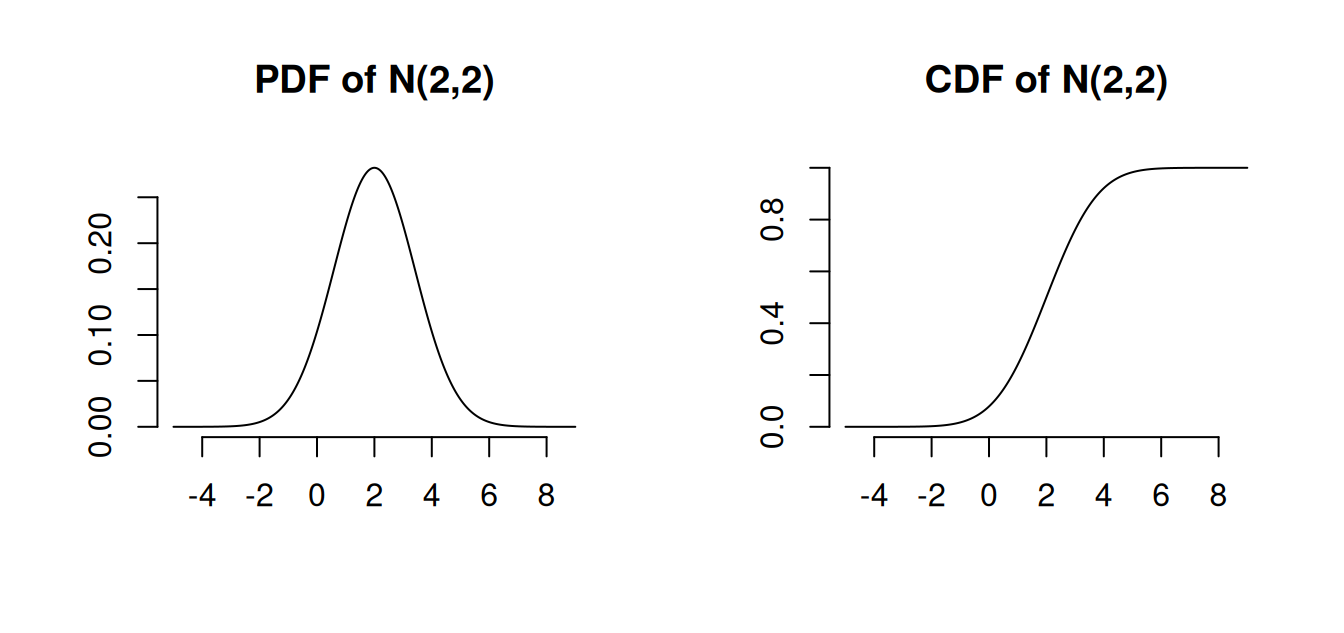
A random variable Z is said to follow a normal distribution if it has the following probability density function (PDF): f(u) = \frac{1}{\sqrt{2 \pi \sigma^2}} \exp\Big(-\frac{(u-\mu)^2}{2 \sigma^2}\Big). Formally, we denote this as Z \sim \mathcal N(\mu, \sigma^2), meaning that Z is normally distributed with mean \mu and variance \sigma^2.
- Mean: E[Z] = \mu
- Variance: \mathrm{Var}(Z) = \sigma^2
- Skewness: \mathrm{skew}(Z) = 0
- Kurtosis: \mathrm{kurt}(Z) = 3
The normal distribution with mean 0 and variance 1 is called the standard normal distribution. It has the PDF \phi(u) = \frac{1}{\sqrt{2 \pi}} \exp\Big(-\frac{u^2}{2}\Big) and its CDF is \Phi(a) = \int_{-\infty}^a \phi(u) \, du. \mathcal N(0,1) is symmetric around zero: \phi(u) = \phi(-u), \quad \Phi(a) = 1 - \Phi(-a)
Standardizing: If Z \sim \mathcal N(\mu, \sigma^2), then \frac{Z-\mu}{\sigma} \sim \mathcal N(0,1). The CDF of Z is P(Z \leq a) = \Phi((a-\mu)/\sigma).
Linear combinations of normally distributed variables are normal: If Y_1, \ldots, Y_n are jointly normally distributed and c_1, \ldots, c_n \in \mathbb R, then \sum_{j=1}^n c_j Y_j is normally distributed.
Multivariate Normal distribution
Let Z_1, \ldots, Z_k be independent \mathcal N(0,1) random variables.
Then, the k-vector \boldsymbol Z = (Z_1, \ldots, Z_k)' has the multivariate standard normal distribution, written \boldsymbol Z \sim \mathcal N(\boldsymbol 0, \boldsymbol I_k). Its joint PDF is f(\boldsymbol x) = \frac{1}{(2 \pi)^{k/2}} \exp\left( - \frac{\boldsymbol x'\boldsymbol x}{2} \right).
If \boldsymbol Z \sim \mathcal N(\boldsymbol 0, \boldsymbol I_k) and \boldsymbol Z^* = \boldsymbol \mu + \boldsymbol B \boldsymbol Z for a q \times 1 vector \boldsymbol \mu and a q \times k matrix \boldsymbol B, then \boldsymbol Z^* has a multivariate normal distribution with mean vector \boldsymbol \mu and covariance matrix \boldsymbol \Sigma = \boldsymbol B \boldsymbol B', written \boldsymbol Z^* \sim \mathcal N(\boldsymbol \mu, \boldsymbol \Sigma).
The q-variate PDF of \boldsymbol Z^* is f(\boldsymbol u) = \frac{1}{(2 \pi)^{q/2} (\det(\boldsymbol \Sigma))^{1/2} } \exp\Big(- \frac{1}{2}(\boldsymbol u-\boldsymbol \mu)'\boldsymbol \Sigma^{-1} (\boldsymbol u-\boldsymbol\mu) \Big).
The mean vector and covariance matrix are E[\boldsymbol Z^*] = \boldsymbol \mu, \quad \mathrm{Var}(\boldsymbol Z^*) = \boldsymbol \Sigma.
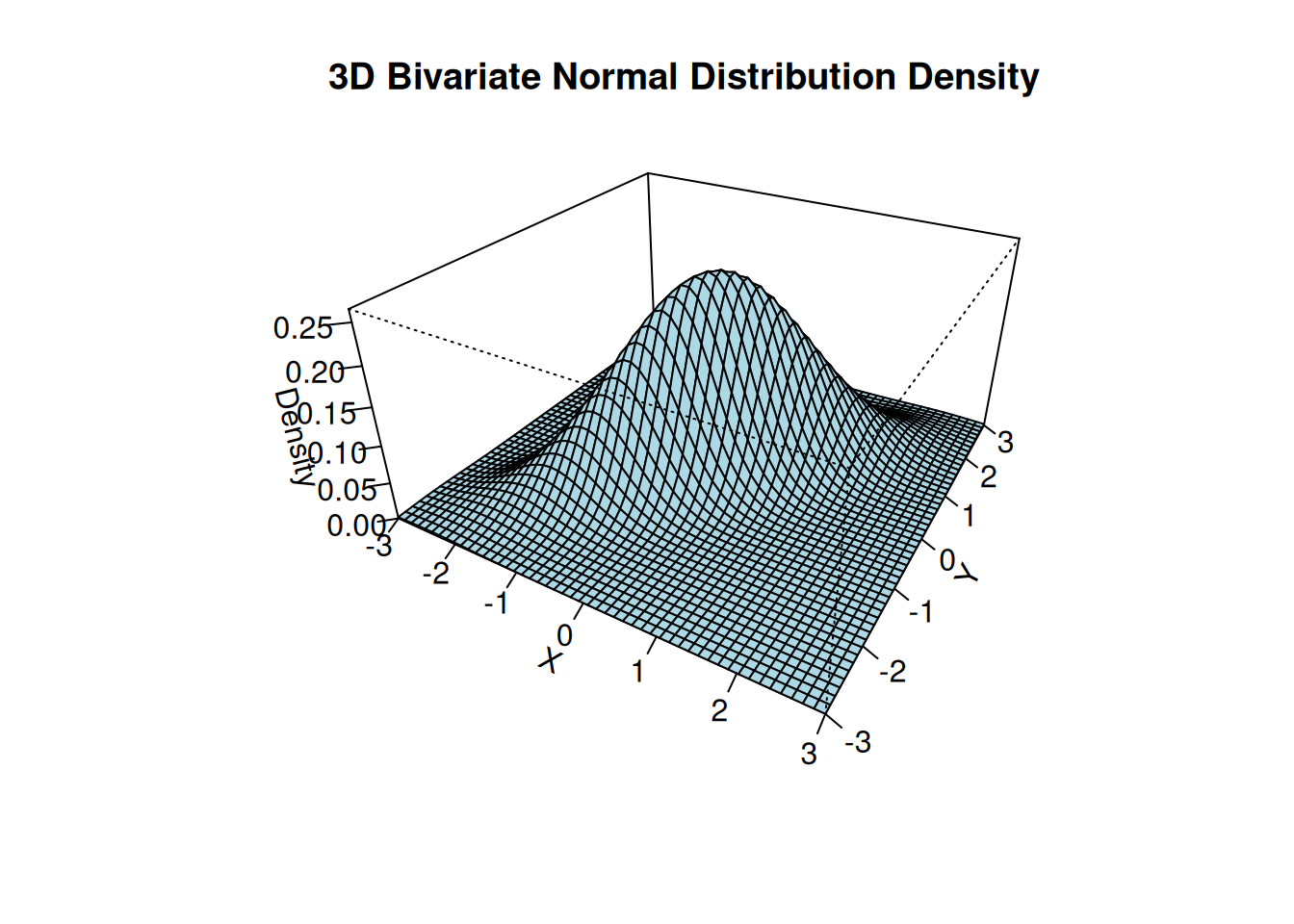
The 3D plot shows the bivariate normal PDF with parameters \boldsymbol \mu = \begin{pmatrix} 0 \\ 0 \end{pmatrix}, \quad \boldsymbol \Sigma = \begin{pmatrix} 1 & 0.8 \\ 0.8 & 1 \end{pmatrix}.
10.4 Central Limit Theorem
Convergence in distribution
Let \boldsymbol V_n be a sequence of k-variate random variables and let \boldsymbol V be a k-variate random variable
\boldsymbol V_n converges in distribution to \boldsymbol V, written \boldsymbol V_n \overset{d}{\rightarrow} \boldsymbol V, if \lim_{n \to \infty} P(\boldsymbol V_n \leq \boldsymbol a) = P(\boldsymbol V \leq \boldsymbol a) for all \boldsymbol a at which the CDF of \boldsymbol V is continuous, where “\leq” is componentwise.
If \boldsymbol V has the distribution \mathcal N(\boldsymbol \mu, \boldsymbol \Sigma), we write \boldsymbol V_n \overset{d}{\rightarrow} \mathcal N(\boldsymbol \mu, \boldsymbol \Sigma).
By the univariate central limit theorem, the sample mean converges to a normal distribution:
Central Limit Theorem (CLT)
Let W_1, \ldots, W_n be an i.i.d. sample with E[W_i] = \mu and \mathrm{Var}(W_i) = \sigma^2 < \infty. Then, the sample mean \overline W = \frac{1}{n}\sum_{i=1}^n W_i satisfies \sqrt n \big( \overline W - \mu \big) \overset{d}{\longrightarrow} \mathcal N(0,\sigma^2).
Below, you will find an interactive shiny app for the central limit theorem:
The same result can be extended to random vectors.
Multivariate Central Limit Theorem (MCLT)
If \boldsymbol W_1, \ldots, \boldsymbol W_n is a multivariate i.i.d. sample with E[\boldsymbol W_i] = \boldsymbol \mu and \mathrm{Var}(\boldsymbol W_i) = \boldsymbol \Sigma < \infty. Then, the sample mean vector \overline{\boldsymbol W} = \frac{1}{n}\sum_{i=1}^n \boldsymbol W_i satisfies \sqrt n \big( \overline{\boldsymbol W} - \boldsymbol \mu \big) \overset{d}{\to} \mathcal N(\boldsymbol 0, \boldsymbol \Sigma) (see, e.g., Stock and Watson Section 19.2).
10.5 Asymptotic Normality
Let’s apply the MCLT to the OLS vector. Consider \boldsymbol W_i = \boldsymbol X_i u_i, which satisfies E[\boldsymbol X_i u_i] = \boldsymbol 0, \quad \mathrm{Var}(\boldsymbol X_i u_i) = E[u_i^2 \boldsymbol X_i \boldsymbol X_i'] = \boldsymbol \Omega.
Therefore, by the MCLT, \sqrt n \bigg( \frac{1}{n} \sum_{i=1}^n \boldsymbol X_i u_i \bigg) \overset{d}{\to} \mathcal N(\boldsymbol 0, \boldsymbol \Omega). Thus, because \frac{1}{n} \sum_{i=1}^n \boldsymbol X_i \boldsymbol X_i' \overset{p}{\to} \boldsymbol Q, \sqrt n (\widehat{\boldsymbol \beta} - \boldsymbol \beta) = \sqrt n \bigg( \frac{1}{n} \sum_{i=1}^n \boldsymbol X_i \boldsymbol X_i' \bigg)^{-1} \bigg( \frac{1}{n} \sum_{i=1}^n \boldsymbol X_i u_i \bigg) \overset{d}{\rightarrow} \boldsymbol Q^{-1} \mathcal N(\boldsymbol 0, \boldsymbol \Omega). where the right-hand side means the distribution of \boldsymbol Q^{-1} \boldsymbol Z for \boldsymbol Z \sim \mathcal N(\boldsymbol 0, \boldsymbol \Omega).
Finally, since the variance of \boldsymbol Q^{-1} \mathcal N(\boldsymbol 0, \boldsymbol \Omega) is \boldsymbol Q^{-1} \boldsymbol \Omega \boldsymbol Q^{-1}, we have the following central limit theorem for the OLS estimator:
Central Limit Theorem for OLS
Consider the linear model Y_i = \boldsymbol X_i' \boldsymbol \beta + u_i such that
- Random sampling: (Y_i, \boldsymbol{X}_i') are i.i.d.
- Exogeneity (mean independence): E[u_i|\boldsymbol X_i] = 0.
- Finite fourth moments: E[X_{ij}^4] < \infty and E[u_i^4] < \infty.
- Full rank: E[\boldsymbol{X}_i\boldsymbol{X}_i'] is positive definite (hence invertible).
Then, as n \to \infty,
\sqrt n (\widehat{\boldsymbol \beta} - \boldsymbol \beta) \overset{d}{\to} \mathcal N(\boldsymbol 0, \boldsymbol Q^{-1} \boldsymbol \Omega \boldsymbol Q^{-1}).
The only additional assumption compared to the consistency of OLS is the finite fourth moments condition instead of the finite second moments condition. This technical assumption ensures that the variance of \boldsymbol X_i u_i is finite.
Specifically, the Cauchy-Schwarz inequality implies that E[X_{ij}^2 u_i^2] \leq \sqrt{E[X_{ij}^4] E[u_i^4]} < \infty, so that the elements of \boldsymbol \Omega are finite.
If homoskedasticity holds, then \boldsymbol \Omega = \sigma^2 \boldsymbol Q, and the asymptotic variance simplifies to \boldsymbol Q^{-1} \boldsymbol \Omega \boldsymbol Q^{-1} = \sigma^2 \boldsymbol Q^{-1}.
10.6 Efficiency
When comparing two unbiased estimators \widehat \theta_n and \widetilde \theta_n then \widehat \theta_n is at least as efficient as \widetilde \theta_n if it has no larger variance: \mathrm{Var}(\widehat \theta_n) \leq \mathrm{Var}(\widetilde \theta_n). For vector-valued estimators, we compare covariance matrices in the Loewner order: \boldsymbol A \preceq \boldsymbol B if \boldsymbol B-\boldsymbol A is a positive semidefinite matrix (see matrix tutorial for details).
Then, the estimator \widehat{ \boldsymbol \theta}_n is at least as efficient as \widetilde{\boldsymbol \theta}_n if the covariance matrices satisfy \mathrm{Var}(\widehat{ \boldsymbol \theta}_n) \preceq \mathrm{Var}(\widetilde{\boldsymbol \theta}_n).
Under homoskedasticity, the OLS coefficient is the efficient estimator for \boldsymbol \beta.
Gauss–Markov Theorem
Consider the linear model Y_i=\boldsymbol X_i'\boldsymbol\beta+ u_i with
- Random sampling: (Y_i,\boldsymbol X_i') i.i.d.
- Exogeneity: E[u_i | \boldsymbol X_i]=0.
- Full rank: \boldsymbol X has column rank k.
- Homoskedasticity: \mathrm{Var}(u_i | \boldsymbol X_i)=\sigma^2.
Then the OLS estimator \widehat{\boldsymbol\beta}=(\boldsymbol X'\boldsymbol X)^{-1}\boldsymbol X'\boldsymbol Y is the Best Linear Unbiased Estimator (BLUE):
- Linear: it is linear in \boldsymbol Y;
- Unbiased: E[\widehat{\boldsymbol\beta}| \boldsymbol X]=\boldsymbol\beta;
- Best: for any other linear unbiased estimator \widetilde{\boldsymbol\beta}, \mathrm{Var}(\widetilde{\boldsymbol\beta} | \boldsymbol X) \ \succeq\ \mathrm{Var}(\widehat{\boldsymbol\beta} | \boldsymbol X) = \sigma^2(\boldsymbol X'\boldsymbol X)^{-1}.
In the heteroskedastic linear regression model, OLS is not efficient. We can recover the Gauss-Markov efficiency in the heteroskedastic linear regression model if we use the generalized least squares estimator (GLS) instead: \begin{align*} \widehat{\boldsymbol \beta}_{gls} &= (\boldsymbol X' \boldsymbol D^{-1} \boldsymbol X)^{-1} \boldsymbol X' \boldsymbol D^{-1} \boldsymbol Y \\ &= \bigg( \sum_{i=1}^n \frac{1}{\sigma_i^2} \boldsymbol X_i \boldsymbol X_i' \bigg)^{-1} \bigg( \sum_{i=1}^n \frac{1}{\sigma_i^2} \boldsymbol X_i Y_i \bigg), \end{align*} where \boldsymbol D = \mathrm{Var}(\boldsymbol u | \boldsymbol X) = \text{diag}(\sigma_1^2, \ldots, \sigma_n^2)
GLS can be derived from the Method of Moments principle using the following moment condition: E[\sigma^{-2}_i \boldsymbol X_i u_i] = E[\sigma^{-2}_i \boldsymbol X_i E[u_i| \boldsymbol X_i]] = \boldsymbol 0. Then E[\sigma^{-2}_i \boldsymbol X_i u_i] = E[\sigma^{-2}_i \boldsymbol X_i (Y_i - \boldsymbol X_i'\boldsymbol \beta)] = \boldsymbol 0 can be rearranged as \boldsymbol \beta = E[\sigma^{-2}_i \boldsymbol X_i \boldsymbol X_i']^{-1} E[\sigma^{-2}_i \boldsymbol X_i Y_i].
The GLS estimator is BLUE in the heteroskedastic linear regression model.
However, GLS is generally infeasible because \boldsymbol D (or the \sigma_i^2) is unknown. Unless we can credibly model \boldsymbol D, the standard approach is to use OLS and account for heteroskedastity in additional inferential steps. When a plausible variance structure is available, one can estimate it and run feasible GLS (FGLS).